Appendix A
Optimization Methods

“Since the building of all the universe is perfect and is created by the wisdom creator, nothing arises in the universe in which one cannot see the sense of some maximum or minimum.”

\(~\) – L. Euler

In this chapter, we give a brief introduction to some of the most basic but important optimization algorithms used in this book. The purpose is only to help the reader apply these algorithms to problems studied in this book, not to gain a deep understanding about these algorithms. Hence, we will not provide a thorough justification for the algorithms introduced, in terms of performance guarantees.

A.1 Steepest Descent

Optimization is concerned with the question of how to find where a function, say \(\cL (\theta )\), reaches its minimum value. Mathematically, this is stated as a problem:

where \(\Theta \) represents a domain to which the argument \(\theta \) is confined. Often (and unless otherwise mentioned, in this chapter) \(\Theta \) is simply \(\R ^{n}\). Without loss of generality, we assume that here the function \(\cL (\theta )\) is smooth¹.

The efficiency of finding the (global) minima depends on what information we have about the function \(\cL \). For most optimization problems considered in this book, the dimension of \(\theta \), say \(n\), is very large. That makes computing or accessing local information about \(\cL \) expensive. In particular, since the gradient \(\nabla \cL \) has \(n\) entries, it is often reasonable to compute; however, the Hessian \(\nabla ^{2} \cL \) has \(n^{2}\) entries which is often wildly impractical to compute (and the same goes for higher-order derivatives). Hence, it is typical to assume that we have the zeroth-order information, i.e., we are able to evaluate \(\cL (\theta )\), and the first-order information, i.e., we are able to evaluate \(\nabla \cL (\theta )\). Optimization theorists may rephrase this as saying we have a “first-order oracle.” All optimization algorithms that we introduce in this section only use a first-order oracle.²

A.1.1 Vanilla Gradient Descent for Smooth Problems

The simplest and most widely used method for optimization is gradient descent (GD). It was first introduced by Cauchy in 1847. The idea is very simple: starting from an initial state, we iteratively take small steps such that each step reduces the value of the function \(\cL (\theta )\).

Suppose that the current state is \(\theta \). We want to take a small step, say of distance \(h\), in a direction, indicated by a vector \(\vv \), to reach a new state \(\theta + h\vv \) such that the value of the function decreases:

To find such a direction \(\vv \), we can approximate \(\cL (\theta + h\vv )\) through a Taylor expansion around \(h = 0\):

where the inner product here (and in this chapter) will be the \(\ell ^{2}\) inner product, i.e., \(\ip {\vx }{\vy } = \vx ^{\top }\vy \). To find the direction of steepest descent, we attempt to minimize this Taylor expansion among unit vectors \(\vv \). If \(\nabla \cL (\theta ) = \vzero \), then the second term above is \(0\) regardless of the value of \(\vv \), so we cannot attempt to make progress, i.e., the algorithm has converged. On the other hand, if \(\nabla \cL (\theta ) \neq \vzero \) then it holds

In words, this means that the value of \(\cL (\theta + h\vv )\) decreases the fastest along the direction \(\vv = -\nabla \cL (\theta ) / \norm {\nabla \cL (\theta )}_{2}\), for small enough \(h\). This leads to the gradient descent method: From the current state \(\theta _{k}\) (\(k=0, 1, \ldots \)), we take a step of size \(h\) in the direction of the negative gradient to reach the next iterate,

The step size \(h\) is also called the learning rate in machine learning contexts.

Step-Size Selection

The remaining question is what the step size \(h\) should be? If we choose \(h\) to be too small, the value of the function may decrease very slowly, as shown by the plot in the middle in Figure A.1. If \(h\) is too large, the value might not even decrease at all, as shown by the plot on the right in Figure A.1.

So the step size \(h\) should be chosen based on the landscape of the function \(\cL (\theta _{k})\). Ideally, to choose the best step size \(h\), we can solve the following optimization problem over a single variable \(h\):

This method of choosing the step size is called line search; as hinted by the notation, it is usually used to obtain an optimal learning rate for each iteration \(k\). However, when the function \(\cL (\theta _{k})\) is complicated, which is usually the case for training a deep neural network, this one-dimensional optimization is very difficult to solve at each iteration of gradient descent.

Then how should we choose a proper step size \(h\)? One common and classical approach is to try to obtain a good approximation of the local landscape around the current state \(\theta \) based on some knowledge about the overall landscape of the function \(\cL (\theta )\).

Common conditions for the landscape of \(\cL (\theta )\) include:

• \(\alpha \)-Strong Convexity. Recall that \(\cL \) is \(\alpha \)-strongly convex if its graph lies above a global quadratic lower bound of slope \(\alpha \), i.e.,

  \begin{equation} \cL (\theta ^{\prime }) \geq l_{\theta , \alpha }(\theta ^{\prime }) \doteq \cL (\theta ) + \ip {\nabla \cL (\theta )}{\theta ^{\prime } - \theta } + \frac {\alpha }{2}\norm {\theta ^{\prime } - \theta }_{2}^{2} \tag{A.1.7} \end{equation}
  for any “base point” \(\theta \). We say that \(\cL \) is convex if it is \(0\)-strongly convex, i.e., its graph lies above its tangents. It is easy to show (proof as exercise) that strongly convex functions have unique global minima. Another important fact (proof as exercise) is that \(\alpha \)-strongly convex twice-differentiable functions \(\cL \) have (symmetric) Hessians \(\nabla ^{2}\cL \) whose minimum eigenvalue is \(\geq \alpha \). For \(\alpha > 0\) this implies the Hessian is symmetric positive definite, and for \(\alpha = 0\) (i.e., \(\cL \) is convex) this implies that the Hessian is symmetric positive semidefinite.

• \(\beta \)-Lipschitz Gradient (also called \(\beta \)-Smoothness). Recall that \(\cL \) has \(\beta \)-Lipschitz gradient if \(\nabla \cL \) exists and is \(\beta \)-Lipschitz, i.e.,

  \begin{equation} \norm {\nabla \cL (\theta ^{\prime }) - \nabla \cL (\theta )}_{2} \leq \beta \norm {\theta ^{\prime } - \theta }_{2}. \tag{A.1.8} \end{equation}
  for any “base point” \(\theta \). It is easy to show (proof as exercise) that this is equivalent to \(\cL \) having a global quadratic upper bound of slope \(\beta \), i.e.,
  \begin{equation} \cL (\theta ^{\prime }) \leq u_{\theta , \beta }(\theta ^{\prime }) \doteq \cL (\theta ) + \ip {\nabla \cL (\theta )}{\theta ^{\prime } - \theta } + \frac {\beta }{2}\norm {\theta ^{\prime } - \theta }_{2}^{2}. \tag{A.1.9} \end{equation}
  for any “base point” \(\theta \). Another important fact (proof as exercise) is that convex \(\beta \)-Lipschitz gradient twice-differentiable functions have (symmetric) Hessians \(\nabla ^{2}\cL \) whose largest eigenvalue is \(\leq \beta \).

First, let us suppose that \(\cL \) has \(\beta \)-Lipschitz gradient (but is not necessarily even convex). We will use this occasion to introduce a common optimization theme: to minimize \(\cL \), we can minimize an upper bound on \(\cL \), which is justified by the following lemma visualized in Figure A.2.

We will use this lemma to show that we can use the Lipschitz gradient property to ensure that each gradient step cannot worsen the value of \(\cL \). Indeed, at every base point \(\theta \), we have that \(u_{\theta , \beta }\) is a global upper bound on \(\cL \), and \(u_{\theta , \beta }(\theta ) = \cL (\theta )\). Hence by Lemma A.1

This motivates us, when finding an update to obtain \(\theta _{k + 1}\) from \(\theta _{k}\), we can instead minimize the upper bound \(u_{\theta _{k}, \beta }\) over \(\theta \) and set that to be \(\theta _{k + 1}\). By minimizing \(u_{\theta _{k}, \beta }\) (proof as exercise) we get

This implies that a step size \(h = 1/\beta \) is a usable learning rate, but it does not provide a convergence rate or certify that \(\cL (\theta _{k})\) actually converges to \(\min _{\theta }\cL (\theta )\). This requires a little more rigor, which we now pursue.

Now, let us suppose that \(\cL \) is \(\alpha \)-strongly convex, has \(\beta \)-Lipschitz gradient, and has global optimum \(\theta ^{\star }\). We will show that \(\theta _{k}\) will converge directly to the unique global optimum \(\theta ^{\star }\), which is a very strong form of convergence. In particular, we will bound \(\norm {\theta ^{\star } - \theta _{k}}_{2}\) using both strong convexity and Lipschitzness of the gradient of \(\cL \), i.e., taking a look at the neighborhood around \(\theta _{k}\):³

In order to ensure that the gradient descent iteration makes progress we must pick the step size so that \(1 - \beta h \geq 0\), i.e., \(h \leq 1/\beta \). If such a setting occurs, then

In order to minimize the right-hand side, we can set \(h = 1/\beta \), which obtains

showing convergence to global optimum with exponentially decaying error. Notice that here we used a convergence rate to obtain a favorable step size of \(h = 1/\beta \). This motif will re-occur in this section.

We end this section with a caveat: learning a global optimum is (usually) impractically hard. Under certain conditions, we can ensure that the gradient descent iterates converge to a local optimum. Also, under more relaxed conditions, we can ensure local convergence, i.e., that the iterates converge to a (global or local) optimum if the sequence is initialized close enough to the optimum.

A.1.2 Preconditioned Gradient Descent for Badly-Conditioned Problems

Newton’s Method

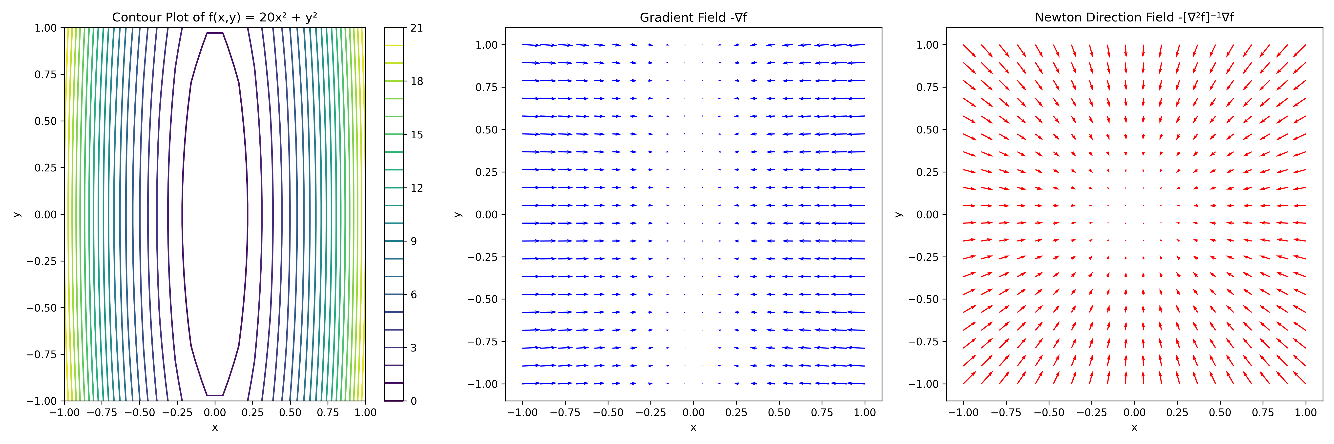
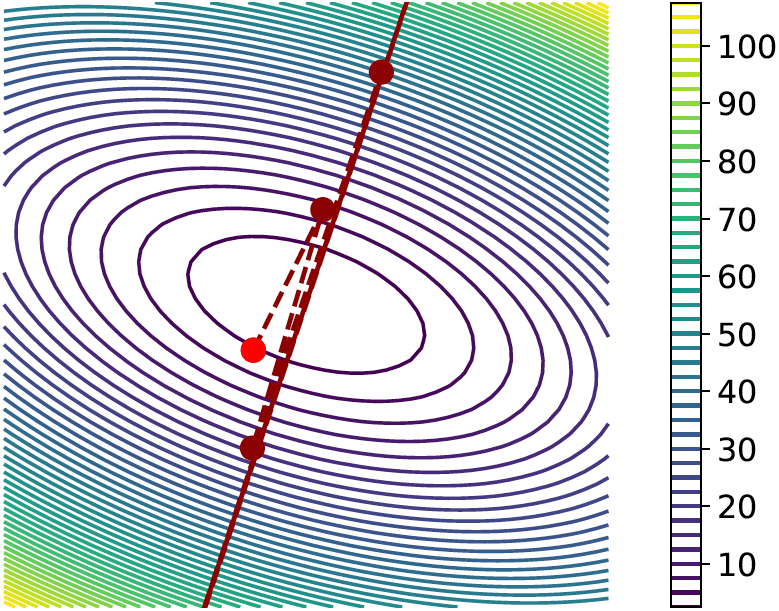
There are some smooth problems and strongly convex problems on which gradient descent nonetheless does quite poorly. For example, let \(\lambda \geq 0\) and let \(\cL _{\lambda } \colon \R ^{2} \to \R \) of the form

This problem is \(1\)-strongly convex and has \((1 + \lambda )\)-Lipschitz gradient. The convergence rate is then geometric with rate \(1 - 1/(1 + \lambda )\). For large \(\lambda \), this is still not very fast. In this section, we will introduce a class of optimization problems which can successfully optimize such badly-conditioned functions.

The key lies in the objective’s curvature, which is given by the Hessian. Suppose that (as a counterfactual) we had a second-order oracle which would allow us to compute \(\cL (\theta )\), \(\nabla \cL (\theta )\), and \(\nabla ^{2}\cL (\theta )\). Then, instead of picking a descent direction \(\vv \) to optimize the first-order Taylor expansion around \(\theta \), we could optimize the second-order Taylor expansion instead. Intuitively this would allow us to incorporate curvature information into the update.

Let us carry out this computation. The second-order Taylor expansion of \(\cL (\theta + h\vv )\) around \(h = 0\) is

Then we can compute the descent direction:

This optimization problem is a little difficult to solve because of the constraint \(\norm {\vv }_{2} = 1\). But in practice we never normalize the descent direction \(\vv \) and use the step size \(h\) to control the size of the update. So let us just solve the above problem over all vectors \(\vv \in \R ^{n}\):⁴

We can thus use the steepest descent iteration

(this is the celebrated Newton’s method), or

(which is called underdamped Newton’s method). Since the second-order quadratic \(\cL _{\lambda }\) is equal to its second-order Taylor expansion, if we run Newton’s method for one step, we will achieve the global minimum in one step no matter how large \(\lambda \) is. Figure A.3 gives some intuition about poorly conditioned functions and the gradient steps versus Newton’s steps.

PGD

In practice, we do not have a second-order oracle which allows us to compute \(\nabla ^{2}\cL (\theta )\). Instead, we can attempt to learn an approximation to it alongside the parameter update \(\theta _{k + 1}\) from \(\theta _{k}\).

How do we learn an approximation to it? We shall find some equations which the Hessian’s inverse satisfies and then try to update our approximation so that it satisfies the equations. Namely, taking the Taylor series of \(\nabla \cL (\theta + \delta _{\theta })\) around point \(\theta \), we obtain

In this case we have

We can now try to learn a symmetric positive semidefinite pre-conditioner \(P \in \R ^{n \times n}\) such that

updating it at each iteration along with \(\theta _{k}\). Namely, we have the PSGD iteration

This update has two problems: how can we even use \(P\) (since we already said we cannot store an \(n \times n\) matrix) and how can we update \(P\) at each iteration? The answers are very related; we can never materialize \(P\) in computer memory, but we can represent it using a low-rank factorization (or comparable methods such as Kronecker factorization which is particularly suited to the form of deep neural networks). Then the preconditioner update step is designed to exploit the structure of the preconditioner representation.

We end this subsection with a caveat: in deep learning, for example, \(\cL \) is not a convex function and so Newton’s method (and approximations to it) do not make sense. In this case we look at the geometric intuition of Newton’s method on convex functions, say from Figure A.3: the inverse Hessian whitens the gradients. Thus instead of a Hessian-approximating preconditioner, we can adjust the above procedures to learn a more general whitening transformation for the gradient. This is the idea behind the original proposal of PSGD [Li17], which contains more information about how to store and update the preconditioner, and more modern optimizers like Muon [LSY+25].

A.1.3 Proximal Gradient Descent for Non-Smooth Problems

Even in very toy problems, however, such as LASSO or dictionary learning, the problem is not strongly convex but rather just convex, and the objective is no longer just smooth but rather the sum of a smooth function and a non-smooth regularizer (such as the \(\ell ^{1}\) norm). Such problems are solved by proximal optimization algorithms, which generalize steepest descent to non-smooth objectives.

Formally, let us say that

where \(\cS \) is smooth, say with \(\beta \)-Lipschitz gradient, and \(\cR \) is non-smooth (i.e., rough). The proximal gradient algorithm generalizes the steepest descent algorithm, by using the majorization-minimization framework (i.e., Lemma A.1) with a different global upper bound. Namely, we construct such an upper bound by asking: what if we take the Lipschitz gradient upper bound of \(S\) but leave \(R\) alone? Namely, we have

Note that (proof as exercise)

Now if we try to minimize the upper bound \(u_{\theta , \beta }\), we are picking a \(\theta ^{\prime }\) that:

• is close to the gradient update \(\theta - \frac {1}{\beta }\nabla \cS (\theta )\);
• has a small value of the regularizer \(\cR (\theta ^{\prime })\)

and trades off these properties according to the smoothness parameter \(\beta \). Accordingly, let us define the proximal operator

Then, we can define the proximal gradient descent iteration which, at each iteration, minimizes the upper bound \(u_{\theta _{k}, h^{-1}}\), i.e.,

Convergence proofs are possible when \(h \leq 1/\beta \), but we do not give any in this section.

One remaining question is: how can we compute the proximal operator? At first glance, it seems like we have traded one intractable minimization problem for another. Since we have not made any assumption on \(\cR \) so far, the framework works even when \(\cR \) is a very complex function (such as a neural network loss), which would require us to solve a neural network training problem in order to compute a single proximal operator. However, in practice, for simple regularizers \(\cR \) such as those we use in this manuscript, there exist proximal operators which are easy to compute or even in closed-form. We give a few below (the proofs are an exercise).

A.1.4 Stochastic Gradient Descent for Large-Scale Problems

In deep learning, the objective function \(\cL \) usually cannot be computed exactly, and instead at each optimization step it is estimated using finite samples (say, using a mini-batch). A common way to model this situation is to define a stochastic loss function \(\cL _{\omega }(\theta )\) where \(\omega \) is some “source of randomness”. For example, \(\omega \) could contain the indices of the samples in a batch over which to compute the loss. Then, we would like to minimize \(\cL (\theta ) \doteq \Ex _{\omega }[\cL _{\omega }(\theta )]\) over \(\theta \), given access to a stochastic first-order oracle: given \(\theta \), we can sample \(\omega \) and compute \(\cL _{\omega }(\theta )\) and \(\nabla _{\theta }\cL _{\omega }(\theta )\). This minimization problem is called a stochastic optimization problem.

The basic first-order stochastic algorithm is stochastic gradient descent: at each iteration \(k\) we sample \(\omega _{k}\), define \(\cL _{k} \doteq \cL _{\omega _{k}}\), and perform a gradient step on \(\cL _{k}\), i.e.,

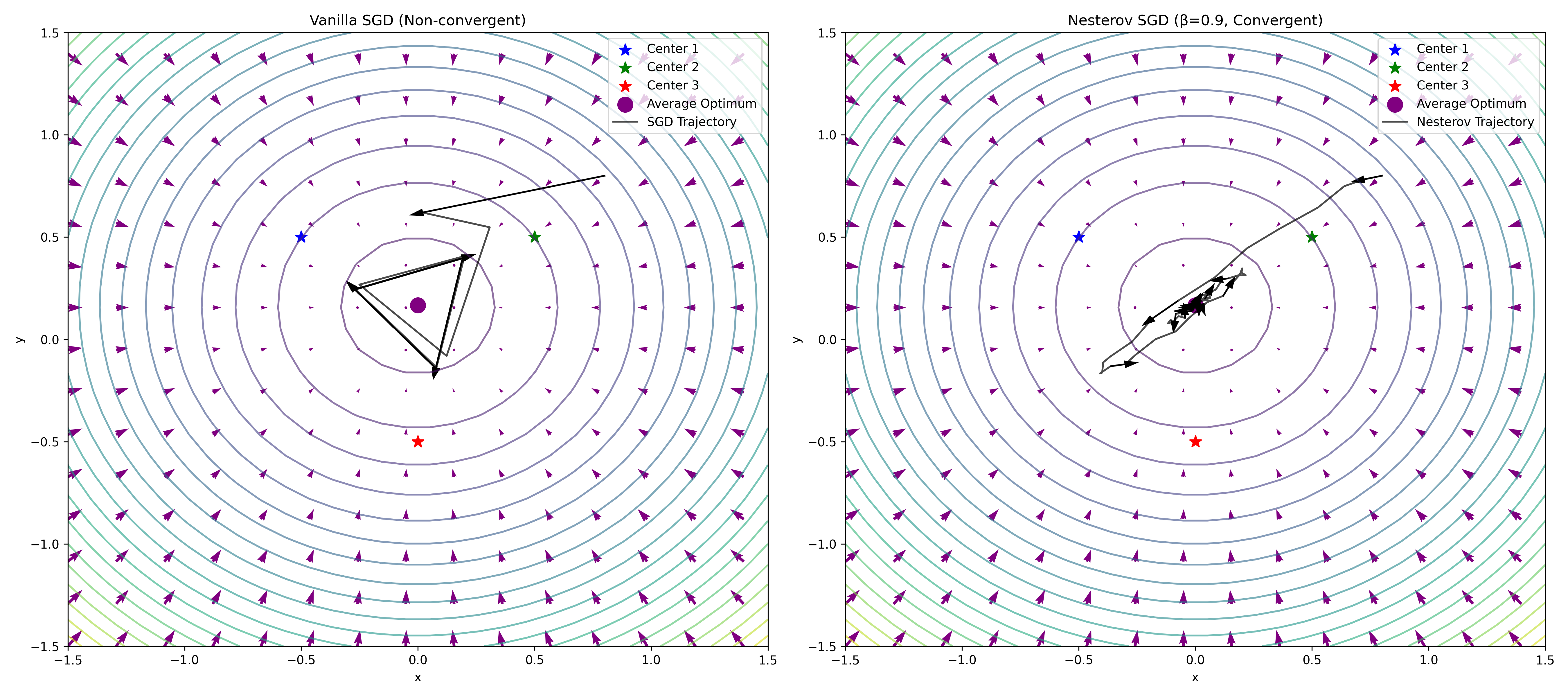
However, even for very simple problems we cannot expect the same type of convergence as we obtained in gradient descent. For example, suppose that there are \(m\) possible values for \(\omega \in \{1, \dots , m\}\) which it takes with equal probability, and there are \(m\) possible targets \(\xi _{1}, \dots , \xi _{m}\), such that the loss function \(\cL _{\omega }\) is

Then \(\argmin _{\theta }\Ex [\cL _{\omega }(\theta )] = \frac {1}{m}\sum _{i = 1}^{m}\xi _{i}\), but stochastic gradient descent can “pinball” around the global optimum value, and not converge, as visualized in Figure A.4.

In order to fix this, we can either average the parameters \(\theta _{k}\) or average the gradients \(\nabla \cL _{k}(\theta _{k})\) over time. If we average the parameters \(\theta _{k}\), then (using Figure A.4 as a mental model) the issue of pinballing is straightforwardly not possible, since the average iterate will grow closer to the center. As such, most theoretical convergence proofs consider the convergence of the average iterate \(\frac {1}{k}\sum _{i = 0}^{k}\theta _{i}\) to the global minimum. If we average the gradients, we will eventually learn an average gradient \(\frac {1}{k}\sum _{i = 0}^{k}\nabla \cL _{k}(\theta _{k})\) which does not change much at each iteration and therefore does not pinball.

In practice, instead of using an arithmetic average, we take an exponentially moving average (EMA) of the parameters (this is called Polyak averaging) or of the gradients (this is called momentum). Momentum is more popular and we will study it here.

A stochastic gradient descent iteration with momentum is as follows:

We do not go through a convergence proof (see Chapter 7 of [GG23] for an example). However, momentum handles our toy case in Figure A.4 easily (see the right-hand figure): it stops pinballing and eventually converges to the global optimum.

We end with a caveat: one can show that Polyak momentum and Nesterov momentum are equivalent, for certain choices of parameter settings. Then it is also possible to show that a decaying learning rate schedule (i.e., the learning rate \(h\) depends on the iteration \(k\), and its limit is \(h_{k} \to 0\) as \(k \to \infty \)) with plain SGD (or PSGD) can mimic the effect of momentum. Namely, [DCM+23] shows that if the SGD algorithm lasts \(K\) iterations, the gradient norms are bounded \(\norm {\nabla \cL (\theta _{k})}_{2} \leq G\), and we define \(D \doteq \norm {\theta _{0} - \theta ^{\star }}_{2}\), then plain SGD iterates \(\theta _{k}\) satisfy the rate \(\Ex [\cL (\theta _{k}) - \cL (\theta ^{\star })] \leq DG/\sqrt {K}\) — but only so long as the learning rate \(h_{k} = (D/[G\sqrt {K}])(1 - k/K)\) decays linearly with time. This matches learning rate schedules used in practice. Indeed, surprisingly, such a theory of convex optimization can predict many empirical phenomena in deep networks [SHT+25], despite deep learning optimization being highly non-convex and non-smooth in the worst case. It is so far unclear why this is the case.

A.1.5 Putting Everything Together: Adam

The gradient descent scheme proposes an iteration of the form

where (recall) \(\vv _{k}\) is chosen to be (proportional to) the steepest descent vector in the Euclidean norm:

However, in the context of deep learning optimization, there is absolutely nothing which implies that we have to use the Euclidean norm; indeed the “natural geometry” of the space of parameters is not well-respected by the Euclidean norm, since small changes in the parameter space can lead to very large differences in the output space, for a particular fixed input to the network. If we were instead to use a generic norm \(\norm {\cdot }\) on the parameter space \(\R ^{n}\), we would get some other quantity corresponding to the so-called dual norm:

For instance, if we were to use the \(\ell ^{\infty }\)-norm, it is possible to show that

where \(\sign (\vx )_{i} = \sign (x_{i}) \in \{-1, 0, 1\}\). Thus if we were so-inclined, we could use the so-called sign-gradient descent:

From sign-gradient descent, we can derive the famous Adam optimization algorithm. Note that for a scalar \(x \in \R \) we can write

Similarly, for a vector \(\vx \in \R ^{n}\) we write (where \(\hada \) and \(\haddiv \) are element-wise multiplication and division)

Using this representation we can write (A.1.53) as

Now consider the stochastic regime where we are optimizing a different loss \(\cL _{k}\) at each iteration. In SGD, we “tracked” (i.e., took an average of) the gradients using momentum. Here, we can track both the gradient and the squared gradient using momentum, i.e.,

where \(\beta ^{i} \in [0, 1]\) are the momentum parameters. The algorithm presented by this iteration is the celebrated Adam optimizer,⁵ which is the most-used optimizer in deep learning. While convergence proofs of Adam are more involved, it falls out of the same steepest descent principle we used so far, and so we should expect that given a small enough learning rate, each update should improve the loss.

Another way to view Adam, which partially explains its empirical success, is that it dynamically updates the learning rates for each parameter based on the squared gradients. In particular, notice that we can write

where \(\eta _{k}\) is the parameter-wise adaptively set learning rate. This scheme is called adaptive because if the gradient of a particular parameter is large up to iteration \(k\), then the learning rate for this parameter becomes smaller to compensate, and vice versa, as can be seen from the above equation.

A.2 Computing Gradients via Automatic Differentiation

Above, we discussed several optimization algorithms for deep networks which assumed access to a first-order oracle, i.e., a device which would allow us to compute \(\cL (\theta )\) and \(\nabla \cL (\theta )\). For simple functions \(\cL \), it is possible to do this by hand. However, for deep neural networks, this quickly becomes tedious, and hinders rapid experimentation. Hence we require a general algorithm which would allow us to efficiently compute the gradients of arbitrary (sub)differentiable network architectures.

In this section, we introduce the basics of automatic differentiation (AD or autodiff ), which is a computationally efficient way to compute gradients and Jacobians of general functions \(f: \R ^{m} \to \R ^{n}\). We will show how this leads to the backpropagation algorithm for computing gradients of loss functions involving neural networks. A summary of the structure of this section is as follows:

1.

We introduce differentials, a convenient formalism for calculating and organizing the derivatives of functions between high-dimensional parameter spaces (which may themselves be products of other spaces involving matrices, tensors, etc.).

2.

We describe the basics of forward-mode and reverse-mode automatic differentiation, which involves considerations that are important for efficient computation of gradients/Jacobians for different kinds of functions arising in machine learning applications.

3.

We describe backpropagation in the special case of a loss function applied to a stack-of-layers neural network as an instantiation of reverse-mode automatic differentiation.

Our treatment will err on the mathematical side, to give the reader a deep understanding of the underlying mathematics. The reader should ensure to couple this understanding with a strong grasp of practical aspects of automatic differentiation for deep learning, for example as manifested in the outstanding tutorial of Karpathy [Kar22b].

A.2.1 Differentials

A full accounting of this subsection is given in the excellent guide [BEJ25]. To motivate differentials, let us first consider the simple example of a differentiable function \(\cL \colon \R \to \R \) acting on a parameter \(\theta \). We can write

If we take \(\delta \theta \doteq \theta ^{+} - \theta \) and \(\delta \cL \doteq \cL (\theta + \delta \theta ) - \cL (\theta )\), we can write

We will (non-rigorously) define \(\odif {\theta }\) and \(\odif {\cL }\), i.e., the differentials of \(\theta \) and \(\cL \), to be infinitesimally small changes in \(\theta \) and \(\cL \). Think of them as what one gets when \(\delta \theta \) (and therefore \(\delta \cL \)) are extremely small. The goal of differential calculus, in some sense, is to study the relationships between the differentials \(\odif {\theta }\) and \(\odif {\cL }\), namely, seeing how small changes in the input of a function change the output. We should note that the differential \(\odif {\theta }\) is the same shape as \(\theta \), and the differential \(\odif {\cL }\) is the same shape as \(\cL \). In particular, we can write

whereby we have that all higher powers of \(\abs {\odif {\theta }}\), such as \((\odif {\theta })^{2}\), are \(0\).

Let’s see how this works for higher dimensions, i.e., \(\cL \colon \R ^{n} \to \R \). Then we still have

for some notion of a derivative \(\cL ^{\prime }(\theta )\). Since \(\theta \) (hence \(\odif {\theta }\)) is a column vector here and \(\cL \) (hence \(\odif {\cL }\)) is a scalar, we must have that \(\cL ^{\prime }(\theta )\) is a row vector. In this case, \(\cL ^{\prime }(\theta )\) is the Jacobian of \(\cL \) w.r.t. \(\theta \). Here notice that we have set all higher powers and products of coordinates of \(\odif {\theta }\) to \(0\). In sum,

All products and powers \(\geq 2\) of differentials are equal to \(0\).

Now consider a higher-order tensor function \(\cL \colon \R ^{m \times n} \to \R ^{p \times q}\). Then our basic linearization equation is insufficient for this case: \(\odif {\cL } = \cL ^{\prime }(\theta ) \cdot \odif {\theta }\) does not make sense since \(\theta \) is an \(m \times n\) matrix but \(\odif {\cL }\) is a \(p \times q\) matrix, so there is no possible vector or matrix shape for \(\cL ^{\prime }(\theta )\) that works in general (as no matrix can multiply a \(m \times n\) matrix to form a \(p \times q\) matrix unless \(m = p\)). So we must have a slightly more advanced interpretation.

Namely, we consider \(\cL ^{\prime }(\theta )\) as a linear transformation whose input is \(\theta \)-space and whose output is \(\cL \)-space, which takes in a small change in \(\theta \) and outputs the corresponding small change in \(\cL \). Namely, we can write

In the previous cases, \(\cL ^{\prime }(\theta )\) was first a linear operator \(\R \to \R \) whose action was to multiply its input by the scalar derivative of \(\cL \) with respect to \(\theta \), and then a linear operator \(\R ^{n} \to \R \) whose action was to multiply its input by the Jacobian derivative of \(\cL \) with respect to \(\theta \). In general \(\cL ^{\prime }(\theta )\) is the “derivative” of \(\cL \) w.r.t. \(\theta \). Think of \(\cL ^{\prime }\) as a generalized version of the Jacobian of \(\cL \). As such, it follows some simple derivative rules, most crucially the chain rule.

It is productive to think of the multivariate chain rule in functorial terms: composition of functions gets ‘turned into’ matrix multiplication of Jacobians (composition of linear operators!). We illustrate the power of this result and this perspective through several examples.

This gives us all the technology we need to compute differentials of everything. The last thing we cover in this section is a method to compute gradients using the differential. Namely, for a function \(\cL \) whose output is a scalar, the gradient \(\nabla \cL \) is defined as

where the inner product here is the “standard” inner product for the specified objects (i.e., for vectors it’s the \(\ell ^{2}\) inner product, whereas for matrices it’s the Frobenius inner product, and for higher-order tensors it’s the analogous sum-of-coordinates inner product). This definition is the correct generalization of the ‘familiar’ example of the gradient of a function from \(\R ^n\) to \(\R \) as the vector of partial derivatives—a version of Taylor’s theorem for general functions \(f : \R ^m \to \R ^n\) makes this connection rigorous. So one way to compute the gradient \(\nabla \cL \) is to compute the differential \(\odif {\cL }\) and rewrite it in the form \(\ip {\text {something}}{\odif {\theta }}\), then that “something” is the gradient.

A.2.2 Automatic Differentiation

The main idea of AD is to compute the chain rule efficiently. The basic problem we need to cope with is the following. In the optimization section of the appendix, we considered that the parameter space \(\Theta \) was an abstract Euclidean space like \(\R ^{n}\). In practice the parameters are really some collection of vectors, matrices, and higher-order objects: \(\Theta = \R ^{m \times n} \times \R ^{n} \times \R ^{r \times q \times p} \times \R ^{r \times q} \times \cdots \). While in theory this is the same thing as a large parameter space \(\R ^{n^{\prime }}\) for some (very large) \(n^{\prime }\), computationally efficient algorithms for differentiation must treat these two spaces differently. Forward and reverse mode automatic differentiation are two different schemes for performing this computation.

Let us do a simple example to start. Let \(\cL \) be defined by \(\cL = a \circ b \circ c\) where \(a, b, c\) are differentiable. Then the chain rule gives

To compute \(\cL (\theta )\), we first compute \(c(\theta )\) then \(b(c(\theta ))\) then \(a(b(c(\theta )))\), and store them all. There are two ways to compute \(\cL ^{\prime }(\theta )\). The forward-mode AD will compute

i.e., computing the derivatives “from the bottom-up”. The reverse mode AD will compute

i.e., computing the derivatives “from the top down”. To see why this matters, suppose that \(f \colon \R ^{p} \to \R ^{s}\) is given by \(f = a \circ b \circ c\) where \(a \colon \R ^{r} \to \R ^{s}\), \(b \colon \R ^{q} \to \R ^{r}\), \(c \colon \R ^{p} \to \R ^{q}\). Then the chain rule is:

where (recall) \(f^{\prime }\) is the derivative, in this case the Jacobian (since the input and output of each function are both vectors). Assuming that computing each Jacobian is trivial and the only cost is multiplying the Jacobians together, forward-mode AD has the following computational costs (assuming that multiplying \(A \in \R ^{m \times n}, B \in \R ^{n \times k}\) takes \(\cO (mnk)\) time):

Meanwhile, doing reverse-mode AD has the following computational costs:

In other words, the forward-mode AD takes \(\cO (p(qr + rs))\) time, and the reverse-mode AD takes \(\cO (s(pq + qr))\) time. These take a different amount of time!

More generally, suppose that \(f = f^{L} \circ \cdots \circ f^{1}\) where each \(f^{\ell } \colon \R ^{d^{\ell - 1}} \to \R ^{d^{\ell }}\), so that \(f \colon \R ^{d^{0}} \to \R ^{d^{L}}\). Then the forward-mode AD takes \(\cO (d^{0}(\sum _{\ell = 2}^{L}d^{\ell - 1}d^{\ell }))\) time while the reverse-mode AD takes \(\cO (d^{L}(\sum _{\ell = 1}^{L - 1}d^{\ell - 1}d^{\ell }))\) time. From the above rates, we see that all else equal:

• If the function to optimize has more outputs than inputs (i.e., \(d^{L} > d^{0}\)), use forward-mode AD.
• If the function to optimize has more inputs than outputs (i.e., \(d^{0} > d^{L}\)), use reverse-mode AD.

In a neural network, we compute the gradient of a loss function \(\cL \colon \Theta \to \R \), where the parameter space \(\Theta \) is usually very high-dimensional. So in practice we always use reverse-mode AD for training neural networks. Reverse-mode AD, in the context of training neural networks, is called backpropagation.

A.2.3 Back Propagation

In this section, we will discuss algorithmic backpropagation using a simple yet completely practical example. Suppose that we fix an input-label pair \((\vX , \vy )\), and fix a network architecture \(f_{\theta } = f_{\theta }^{L} \circ \cdots \circ f_{\theta }^{1} \circ f_{\theta }^{\emb }\) where \(\theta = (\theta ^{\emb }, \theta ^{1}, \dots , \theta ^{L}, \theta ^{\head })\) and task-specific head \(h_{\theta ^{\head }}\), and write

Then, we can define the loss on this one term by

where \(\sfL \) is a differentiable function of its second argument. Then the backward-mode AD instructs us to compute the derivatives in the order \(\theta ^{\head }, \theta ^{L}, \dots , \theta ^{1}, \theta ^{\emb }\).

To carry out this computation, let us make some changes to the notation.

• First, let us change the notation to emphasize the dependency structure between the variables. Namely,

  \begin{align} &\vZ ^{1} \doteq f^{\emb }(\vX , \theta ^{\emb }) \tag{A.2.42} \\ &\vZ ^{\ell + 1} \doteq f^{\ell }(\vZ ^{\ell }, \theta ^{\ell }), \qquad \forall \ell \in \{1, \dots , L\}, \tag{A.2.43} \\ &\hat {\vy } \doteq h(\vZ ^{L+1}, \theta ^{\head }), \tag{A.2.44} \\ &\cL \doteq \sfL (\vy , \hat {\vy }). \tag{A.2.45} \end{align}
• Then, instead of having the derivative be \(f^{\prime }\), we explicitly notate the independent variable and write the derivative as \(\odv {f}{\theta ^{1}}\), for example. This is because there are many variables in our model and we only care about one at a time.

We can start by computing the appropriate differentials. First, for \(\theta ^{\head }\) we have

Now since \(\vZ ^{L + 1}\) does not depend on \(\theta ^{\head }\), we have \(\odif {\vZ }^{L + 1} = 0\), so in the end it holds (using the fact that the gradient is the transpose of the derivative for a function \(\sfL \) whose codomain is \(\R \)):

Thus to compute \(\nabla _{\theta ^{\head }}\cL \), we compute the gradient \(\nabla _{\hat {\vy }}\sfL \) and the adjoint⁶ of the derivative \(\odv {h}{\theta ^{\head }}\) and multiply (i.e., apply the adjoint linear transformation to the gradient). In practice, both derivatives can be computed by hand, but many modern computational frameworks can automatically define the derivatives (and/or their adjoints) given code for the “forward pass,” i.e., the loss function computation. While extending this automatic derivative definition to as many functions as possible is an area of active research, the resource [BEJ25] describes one basic approach to do it in some detail. By the way, backpropagation is also called the adjoint method for this reason — i.e., that we use adjoint derivatives to compute the gradient.

Now let us compute the differentials w.r.t. some \(\theta ^{\ell }\):

Thus to compute \(\nabla _{\theta ^{\ell }}\cL \) we compute \(\nabla _{\vZ ^{\ell + 1}}\cL \) then apply the adjoint derivative \(\bp {\odv {f^{\ell }}{\theta ^{\ell }}}^{*}\) to it. Since \(\nabla _{\theta ^{\ell }}\cL \) depends on \(\nabla _{\vZ ^{\ell + 1}}\cL \), we also want to be able to compute the gradients w.r.t. \(\vZ ^{\ell }\). This can be computed in the exact same way:

Thus to compute \(\nabla _{\vZ ^{\ell }}\cL \) we compute \(\nabla _{\vZ ^{\ell + 1}}\cL \) then apply the adjoint derivative \(\bp {\odv {f^{\ell }}{\vZ ^{\ell }}}^{*}\) to it. So we have a recursion to compute \(\nabla _{\vZ ^{\ell }}\cL \) for all \(\ell \), with base case \(\nabla _{\vZ ^{L + 1}}\cL \), which is given by

Thus we have the recursion:

This gives us a computationally efficient algorithm to find all gradients in the whole network.

We’ll finish this section by computing the adjoint derivative for a simple layer.

Note that as a simple application of chain rule, both backpropagation and automatic differentiation work over general “computational graphs”, i.e., compositions of (simple) functions. We give all examples as neural network layers because this is the most common example in practice.

A.3 Game Theory and Minimax Optimization

In certain cases, such as in Chapter 6, a learning problem cannot be reduced to a single optimization problem but rather represents multiple potentially opposing components of the system trying to each minimize their own objective. Examples of this paradigm include distribution learning via generative adversarial networks (GAN) and closed-loop transcription (CTRL). We will denote such a system as a two-player game, where we have two “players” (i.e., components) called Player 1 and Player 2 trying to minimize their objectives \(\cL ^{1}\) and \(\cL ^{2}\) respectively. Player 1 picks parameters \(\theta \in \Theta \) and Player 2 picks parameters \(\eta \in \Eta \). In this book we consider the special case of zero-sum games, i.e., defining a common objective \(\cL \) such that \(\cL = -\cL ^{1} = \cL ^{2}\).

Our first, very preliminary example is as follows. Suppose that there exists functions \(u(\theta )\) and \(v(\eta )\) such that

Then both players’ objectives are independent of the other player, and the players should try to achieve their respective optima:

The pair \((\theta ^{\star }, \eta ^{\star })\) is a straightforward special case of an equilibrium: a situation where neither player will want to move, given the chance, since moving will end up making their own situation worse. However, not all games are so trivial; many have more complicated objectives and information structures.

In this book, the relevant game-theoretic formalism is a Stackelberg game (variously called sequential game). In this formalism, one player (without loss of generality Player 1, and also described as a leader) picks their parameters before the other (i.e., Player 2, also described as a follower), and the follower can use the full knowledge of the leader’s choice to make their own choice. The correct notion of equilibrium for a Stackelberg game is a Stackelberg equilibrium. To explain this equilibrium, note that since Player 2 (i.e., the follower) can choose \(\eta \) reactively to the choice \(\theta _{1}\) made by Player 1 (i.e., the leader), Player 2 would of course choose the \(\eta \) which minimizes \(\cL (\theta _{1}, \cdot )\). But of course a rational Player 1 would realize this, and so pick a \(\theta _{1}\) such that the worst-case \(\eta \) picked by Player 2 according to this rule is not too bad. More formally, let \(\cS (\theta ) \doteq \argmin _{\eta \in \Eta }\cL (\theta , \eta )\) be the set of \(\eta \) minimizing \(\cL (\theta , \eta )\), i.e., the set of all \(\eta \) which Player 2 is liable to play given that Player 1 has played \(\theta \). Then \((\theta ^{\star }, \eta ^{\star })\) is a Stackelberg equilibrium if

Actually (proof as exercise), one can show that in the context of two-player zero-sum Stackelberg games, \((\theta ^{\star }, \eta ^{\star })\) is a Stackelberg equilibrium if and only if

(note that the notation \(\cS (\theta )\) is not used nor needed).

In the rest of the section, we will briefly discuss some algorithmic approaches to learn Stackelberg equilibria. The intuition you should have is that learning an equilibrium is like letting the different parts of the system automatically figure out tradeoffs between the different objectives they want to optimize.

We end this section with a caveat: in two-player zero-sum games, if it holds that

then every Stackelberg equilibrium is a saddle point,⁷ i.e.,

and vice versa, and furthermore each Stackelberg equilibrium has the (same) objective value

Conditions under which the \(\min \max = \max \min \) equality holds are given by so-called minimax theorems; the most famous of these is a theorem of von Neumann. However, in the cases we think about, this property usually does not hold.

A.3.1 Learning Stackelberg Equilibria

How can we learn Stackelberg equilibria via GDA? In general this is clearly impossible, since learning Stackelberg equilibria via GDA is obviously at least as hard as computing a global minimizer of a loss function (say by setting the shared objective \(\cL (\theta , \eta )\) to only be a function of \(\eta \)). As such, we can achieve two types of convergence guarantees:

• When \(\cL \) is (strongly) concave in the first argument \(\theta \) and (strongly) convex in the second argument \(\eta \) (as well as having Lipschitz gradients in both arguments), we can achieve exponentially fast convergence to a Stackelberg equilibrium.
• When \(\cL \) is not concave or convex in either argument, we can achieve local convergence guarantees: namely, if we initialize the parameter values near a (local) Stackelberg equilibrium and the optimization geometry is good then we can learn that equilibrium efficiently.

The former situation is exactly analogous to the case of single-player optimization, where we proved that gradient descent converges exponentially fast for strongly convex objectives which have Lipschitz gradient. The latter situation is also analogous to the case of single-player optimization, although we did not cover it in depth due to technical difficulty; indeed there exist local convergence guarantees for nonconvex objectives which have locally nice geometry.

The algorithm in these two cases is the same algorithm, called Gradient Descent-Ascent (GDA). To motivate GDA, suppose we are trying to learn \(\theta ^{\star }\). We could do gradient ascent on the function \(\theta \mapsto \min _{\eta \in \Eta }\cL (\theta , \eta )\). But then we would need to take the derivative in \(\theta \) of this function. To see how to do this, suppose that \(\cL \) is strongly convex in \(\eta \) so that there is one minimizer \(\eta ^{\star }(\theta )\) of \(\cL (\theta , \cdot )\). Then, Danskin’s theorem says that

where the gradient is only with respect to the first argument (i.e., not a total derivative which would require computing the Jacobian of \(\eta ^{\star }(\theta )\) with respect to \(\theta \)), indicated by the stop-gradient operator.⁸ In order to take the derivative in \(\theta \), we need to set up a secondary process to also optimize \(\eta \) to obtain an approximation for \(\eta ^{\star }(\theta )\). We can do this through the following algorithmic template:

That is, we take \(T\) steps of gradient descent to update \(\eta _{k}\) (hopefully to the minimizer of \(\cL (\theta _{k}, \cdot )\)), and then take a gradient ascent step to update \(\theta _{k}\). As a bonus, on top of estimating \(\theta _{K} \approx \argmax _{\theta }\min _{\eta }\cL (\theta , \eta )\), we also learn an \(\eta _{K} \approx \argmin _{\eta }\cL (\theta _{K}, \eta )\) — this is an approximate Stackelberg equilibrium.

This method is often not done in practice, as it requires \(T + 1\) total gradient descent iterations to update \(\theta \) once. Instead, we use the so-called (simultaneous) Gradient Descent-Ascent (GDA) iteration

which can be implemented efficiently via a single gradient step on \((\theta , \eta )\). The crucial idea here is, to make our method close to the inefficient iteration above, we use an \(\eta \) update which is \(T\) times faster than the \(\theta \) update (these can be seen as nearly the same by taking a linearization of the dynamics).

It is crucial to pick \(T\) sensibly. How can we do that? In the sequel, we discuss two configurations of \(T\) which lead to convergence of GDA to a Stackelberg equilibrium under different assumptions.

Convergence of One-Timescale GDA to Stackelberg Equilibrium

If \(T = 1\) (i.e., named one-timescale because both \(\theta \) and \(\eta \) updates are of the same scale), then the GDA algorithm becomes

If \(\cL \) has Lipschitz gradients in \(\theta \) and \(\eta \), and is strongly concave in \(\theta \) and strongly convex in \(\eta \), and is coercive (i.e.,\(\lim _{\norm {\theta }_{2}, \norm {\eta }_{2} \to \infty }\cL (\theta , \eta ) = \infty \)), then all saddle points are Stackelberg equilibria and vice versa. The work [ZAK24] shows that GDA (again, with \(T = 1\)) with sufficiently small step size \(h\) converges to a saddle point (hence Stackelberg equilibrium) exponentially fast if one exists, analogously to gradient descent for strongly convex functions with Lipschitz gradient.⁹ To our knowledge, this flavor of results constitute the only known rigorous justification for single-timescale GDA.

Local Convergence of Two-Timescale GDA to Stackelberg Equilibrium

Strong convexity/concavity is a global property, and none of the games we look into in this book have objectives which are globally strongly concave/strongly convex. In this case, the best we can hope for is local convergence to Stackelberg equilibria: if the parameters are initialized close to a Stackelberg equilibrium, then GDA can converge onto it, given an appropriate step size \(h\) and timescale \(T\).

In fact, our results also hold for a version of the local Stackelberg equilibrium called the differential Stackelberg equilibrium, which was introduced in [FCR19] (though we use the precise definition in [LFD+22]), and which we define as follows. A point \((\theta ^{\star }, \eta ^{\star })\) is a differential Stackelberg equilibrium if:

• \(\nabla _{\eta }\cL (\theta ^{\star }, \eta ^{\star }) = \vzero \);
• \(\nabla _{\eta }^{2}\cL (\theta ^{\star }, \eta ^{\star })\) is symmetric positive definite;
• \(\nabla _{\theta }\cL (\theta ^{\star }, \eta ^{\star }) = \vzero \);
• \((\nabla _{\theta }^{2}\cL + [\frac{\mathrm{d}}{\mathrm{d}\theta } \nabla _{\eta }\cL ][\nabla _{\eta }^{2}\cL ]^{-1}[\frac{\mathrm{d}}{\mathrm{d}\eta } \nabla _{\theta }\cL ])(\theta ^{\star }, \eta ^{\star })\) is symmetric negative definite.

Notice that the last condition asks for the (total) Hessian

or, equivalently, its Schur complement to be negative definite. If we look at the computation of \(\nabla _{\theta }[\min _{\eta \in \Eta }\cL (\theta , \eta )]\) furnished by Danskin’s theorem, the last two criteria are actually constraints on the gradient and Hessian of the function \(\theta \mapsto \min _{\eta \in \Eta }\cL (\theta , \eta )\), ensuring that the gradient is \(0\) and the Hessian is negative semidefinite. This intuition tells us that we can expect that each Stackelberg equilibrium is a differential Stackelberg equilibrium; [FCR20] confirms this rigorously (up to some technical conditions).

Analogously to the notion of strict local optimum in single-player optimization (where we require \(\nabla ^{2}\cL (\theta ^{\star })\) to be positive semidefinite), the definition of differential Stackelberg equilibrium implies that \(\cL (\theta , \cdot )\) is locally (strictly) convex in a neighborhood of the equilibrium, and that \(\min _{\eta \in \Eta }\cL (\cdot , \eta )\) is locally (strictly) concave in the same region.

In this context, we present the result from [LFD+22]. Let \((\theta ^{\star }, \eta ^{\star })\) be a differential Stackelberg equilibrium. Suppose that \(\cL \) has Lipschitz gradients, i.e.,

Further define the local strong convexity/concavity parameters of \(\cL (\theta , \cdot )\) and \(\min _{\eta }\cL (\cdot , \eta )\) respectively as

Then define the local condition numbers as

The paper [LFD+22] says that if we take step size \(h = \frac {1}{4\beta T}\) and take \(T \geq 2\kappa _{\eta }\), so that the algorithm is

the total Hessian \(\nabla ^{2}\cL (\theta ^{\star }, \eta ^{\star })\) is diagonalizable, and we initialize \((\theta _{0}, \eta _{0})\) close enough to \((\theta ^{\star }, \eta ^{\star })\), then there are positive constants \(c_{0}, c_{1} > 0\) such that

implying exponential convergence to the differential Stackelberg equilibrium.

A.3.2 Practical Considerations when Learning Stackelberg Equilibria

In practice, we do not know how to initialize parameters close to a (differential) Stackelberg equilibrium. Due to symmetries within the objective, including those induced by overparameterization of the neural networks being trained, one can (heuristically) expect that most initializations are close to a Stackelberg equilibrium. Also, we do not know how to compute the step size \(h\) or the timescale \(T\), since they are dependent on properties of the loss \(\cL \) at the equilibrium. In practice, there are some common approaches:

• Take \(T = 1\) (equal step-sizes), and use updates for \(\theta \) and \(\eta \) that are derived from a learning-rate-adaptive optimizer like Adam (as opposed to vanilla GD). Here, you hope (but do not know) that the optimizer can adjust the learning rates to learn a good equilibrium.
• Take \(T\) to be some constant like \(T = 10^{6}\) which implies that \(\eta \) equilibrates \(10^{6}\) times as fast as \(\theta \). Here you can also use Adam-style updates, and hope that it fixes the time scale.
• Let \(T\) depend on the iteration \(k\), and let \(T_{k} \to \infty \) as \(k \to \infty \). This schedule was studied (also in the case of noise) by Borkar in [Bor97].

For example, you can use this while training CTRL-style models (see Chapter 6), where the encoder is Player \(1\) and the decoder is Player \(2\). Some theory about CTRL is given in Theorem 6.1.

A.4 Exercises