“When you can measure what you are speaking about and express it in numbers, you know something about it; but when you cannot measure it, when you cannot express it in numbers, your knowledge is of the meager and unsatisfactory kind: it may be the beginning of knowledge, but you have scarcely, in your thoughts, advanced to the stage of science, whatever the matter may be.”
\(~\) – Lord Kelvin, 1883
Let us recap what we have covered so far. We have shown that it is possible to identify and access a distribution with arbitrary low-dimensional support, such as the one illustrated in Figure 4.1 (left), by gradually transforming the distribution of pure noise (high entropy) into the distribution to be learned via iterative denoising. We have shown that the denoiser at each iteration is directly connected to the gradient of the distribution’s log-density via Tweedie’s formula (3.2.23). We showed that in practice such a denoiser \(\bar {\vx }_{\theta }\) can be estimated using finite samples. Thus we developed a general way of learning or pursuing a data distribution.
Nevertheless, in this methodology the encoding of the distribution is implicit in the denoiser’s functional form and parameters, if any. In fact, acute readers might have noticed that for a general distribution we have never explicitly specified what the functional form for the denoiser should be. In practice, people typically model it with some deep neural network that has an empirically designed architecture. In addition, although we know the above denoising process reduces the entropy, we do not know by how much, nor do we know the entropy of the intermediate and resulting distributions. Hence it would be very useful to know the (optimal) form of the denoising operation and how to measure the change in entropy. Finally, we showed at the end of the last Chapter that if the denoising process reduces the entropy too much it leads to learning only the training data, with no possible interpolation or extrapolation. The methodological innovation which resolves all of these issues will be developed in the Chapter to come.
Measure of information. Recall that our general goal is to model data from a continuous distribution with low-dimensional support. If we want to identify the simplest model that generates the data, we might consider three typical measures of parsimony: dimension, volume, or differential entropy. If we use dimension, then obviously the best model for a given dataset is the empirical distribution itself, which is zero-dimensional.1 If we use the entropy of the data instead, then for all distributions with low-dimensional support, the differential entropy is always negative infinity. Or if we use the volume of the space spanned by the data, the volume of the support of any low-dimensional model is always zero. So, among all distributions with low-dimensional support that could have generated the same data samples, how can we decide which one is better based on these measures of parsimony that cannot distinguish among themselves at all?
In this Chapter, we discuss a framework that alleviates the above technical difficulty by associating the learned distribution with an explicit computable encoding and decoding scheme, following and making more explicit the second approach suggested at the end of Section 3.1.3. As we will see, such an approach essentially allows us to accurately approximate the entropy of the learned distributions in terms of a lossy coding rate associated with the coding scheme, as described and motivated (but not formalized) at the end of Section 3.3. Roughly speaking, such a measure can be viewed as a generalized notion of volume of the empirical data distribution. With such a measure, we can accurately quantify how much the entropy is reduced through a transformation of the distribution, say by a denoiser. In addition, with such a measure, we can derive, at least in principle, the optimal denoising operator that reduces the entropy the fastest.
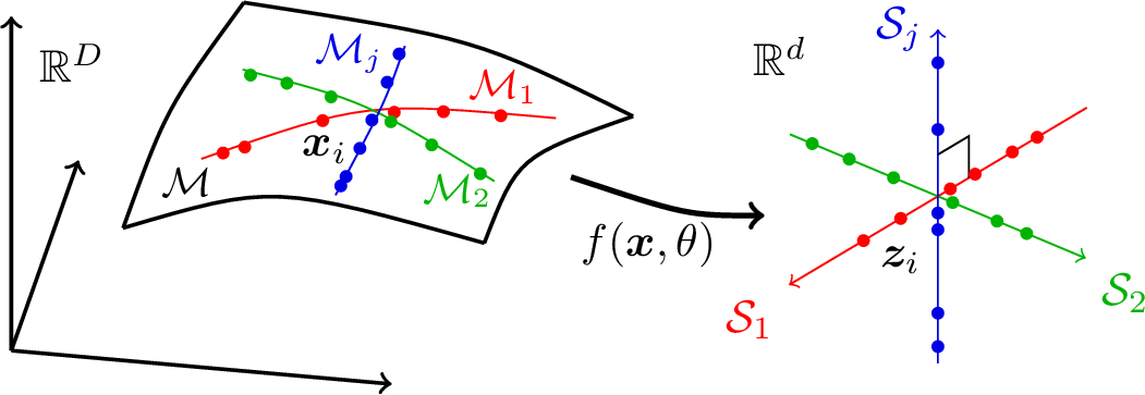
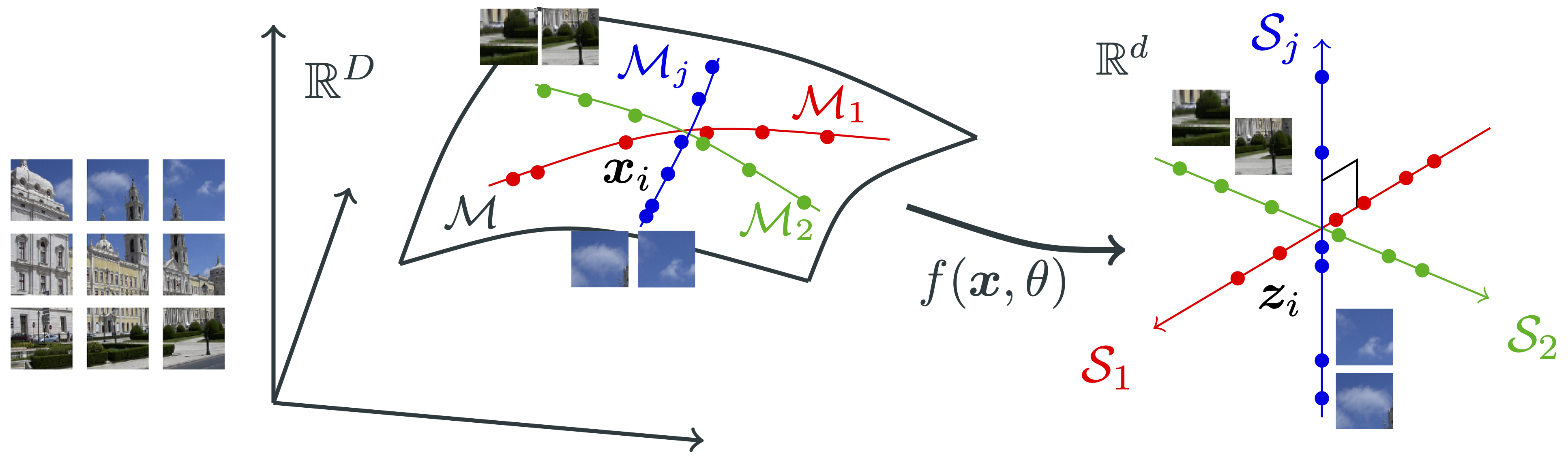
Representation learning. Even though the diffusion and denoising process introduced in the previous chapter allows us, in principle, to learn an arbitrary low-dimensional distribution, it does not give an explicit representation of the distribution. As we will see, the learned distribution is to be repeatedly accessed and used for subsequent tasks (such as used as the prior for Bayesian inference in Chapter 7). Hence it is desirable that we can transform the data distribution, say by a mapping \(f(\vx ,\theta )\), to some standard structured form that facilitates efficient access, say a mixture of (incoherent) linear subspaces or low-rank Gaussians, as illustrated in Figure 4.1 right. We will formalize this process as “representation learning” in this Chapter.
As we will also see, for an arbitrary distribution, the above measure of information (coding rate) is not (easily) computable. But for a mixture of subspaces or low-rank Gaussians, we can derive an accurate closed form for the measure. By optimizing this measure, it will allow us to find the optimal representation. As we will see in the next Chapter 5, optimizing the measure also allows us to derive explicit forms of the operator that performs the transformation \(f(\vx ,\theta )\) in the most efficient way. This will lead to a principled explanation for the architecture of deep networks, as well as to more efficient deep-architecture designs.
In this section, we develop the lossy coding rate as a computable measure of complexity for distributions with low-dimensional support—a setting where classical measures such as entropy, dimension, and volume all fail to distinguish among candidate models. We first motivate the necessity of lossy coding with respect to these pathologies (Section 4.1.1), then show that the rate distortion function connects this coding-theoretic measure to the geometry of the data support via sphere covering (Theorem 4.1). This connection is the bridge between information-theoretic and geometric approaches to learning low-dimensional distributions. Finally, we develop a tight closed-form approximation to the lossy coding rate for Gaussians (Section 4.1.3) and an effective algorithm for clustering mixtures of low-dimensional Gaussians (Section 4.1.4), which will be generalized to nonlinear distributions in the following section.
We have previously, multiple times, discussed a difficulty: if we learn the distribution from finite samples in the end, and our function class of denoisers contains enough functions, how do we ensure that we sample from the true distribution (with low-dimensional supports), instead of any other distribution that may produce those finite samples with high probability? Let us reveal some of the conceptual and technical difficulties with some concrete examples.
Example 4.1 (Volume, Dimension, and Entropy). For the example shown on the top of Figure 4.2, suppose we have taken some samples from a uniform distribution on a line (say in a 2D plane). The volume of the line or the sample sets is zero. Geometrically, the empirical distribution on the produced finite sample set is the minimum-dimension one which can produce the finite sample set.2 But this is in seemingly contrast with yet another measure of complexity: entropy. The (differential) entropy of the line is negative infinity but the (discrete) entropy of this sample set is finite and positive. So we seem to have a paradoxical situation according to these common measures of parsimony or complexity: they cannot properly differentiate among (models for) distributions of low-dimensional supports at all, and some seem to differentiate them even in exactly opposite manners.3 \(\blacksquare \)
Example 4.2 (Density). Consider the two sets of sampled data points shown in Figure 4.2. Geometrically, they are essentially the same: each set consists of eight points and each point has occurred with equal frequency \(1/8\)th. The only difference is that for the second data set, some points are “close” enough to be viewed as having a higher density around their respective “cluster.” Which one is more relevant to the true distribution that may have generated the samples? How can we reconcile such ambiguity in interpreting this kind of (empirical) distributions?

There is yet another technical difficulty associated with constructing an explicit encoding and decoding scheme for a data set. Given a sampled data set in \(\vX = [\vx _1, \ldots , \vx _N]\), how to design a coding scheme that is implementable on machines with finite memory and computing resources? Note that even representing a general real number requires an infinite number of digits or bits. Therefore, one may wonder whether the entropy of a distribution is a direct measure for the complexity of its (optimal) coding scheme. We examine this matter with another simple example.
Example 4.3 (Precision). Consider a discrete distribution \(\vX = [e, \pi ]\) with equal probability \(1/2\) taking the values of the Euler number \(e \approx 2.71828\) or the number \(\pi \approx 3.14159\). The entropy of this distribution is \(H =1\), which suggests that one may encode the two numbers by a one-bit digit \(0\) or \(1\), respectively. But can you realize a decoding scheme for this code on a finite-state machine? The answer is actually no, as it takes infinitely many bits to describe either number precisely. \(\blacksquare \)
Hence, it is generally impossible to have an encoding and decoding scheme that can precisely reproduce samples from an arbitrary real-valued distribution.4 But there would be little practical value to encode a distribution without being able to decode for samples drawn from the same distribution.
So to ensure that any encoding/decoding scheme is computable and implementable with finite memory and computational resources, we need to quantify the sample \(\vx \) and encode it only up to a certain precision, say \(\epsilon > 0\). By doing so, in essence, we treat any two data points as equivalent if their distance is less than \(\epsilon \). More precisely, we would like to consider coding schemes
such that the expected error caused by the quantization is bounded by \(\epsilon \). It is mathematically more convenient, and conceptually almost identical, to bound the expected squared error by \(\epsilon ^{2}\), i.e.,
Typically, the distance \(d\) is chosen to be the Euclidean distance, or the 2-norm.5 We will adopt this choice in the sequel.
Of course, among all encoding schemes that satisfy the above constraint, we would like to choose the one that minimizes the resulting coding rate. For a given random variable \(\vx \) and a precision \(\epsilon \), this rate is known as the rate distortion, denoted as \(\cR _{\epsilon }(\vx )\).
To understand this rate distortion better, we turn to a deep theorem of information theory, originally proved in Shannon [Sha59], which relates this rate distortion to other information-theoretic quantities. To understand this theorem, we first need to define a measure of difference between two distributions known as the Kullback-Leibler (KL) divergence, or relative entropy, which is denoted by \(\KL (\cdot \mmid \cdot )\) and defined in relation to the entropy and cross-entropy (see Section 3.1.3) as
The KL divergence is always non-negative, and equals zero if and only if \(p = q\);6 in the case where \(p\) and \(q\) have the same support and both are probability densities, this can be proved by the following calculation based on Jensen’s inequality and the fact that the function \(\log (\cdot )\) is strictly concave:
Then, we define the mutual information \(I(\cdot ; \cdot )\), which is a measure of dependence between two random variables, as
With the previous definitions in place, we may write the rate distortion \(\cR _{\epsilon }\) in purely probabilistic terms as
Note that the minimization in (4.1.9) is over all conditional distributions \(p(\hat \vx \mid \vx )\) that satisfy the distortion constraint \(\Ex [\norm {\vx - \hat \vx }_2^{2}] \le \epsilon ^{2}\). Each such conditional distribution induces a joint distribution \(p(\vx , \hat {\vx }) = p(\hat \vx \mid \vx ) p(\vx )\), which determines the mutual information (4.1.8). Many convenient properties of the mutual information (and hence the rate distortion) are implied by corresponding properties of the KL divergence. From the definition, we know that \(\cR _{\epsilon }(\vx )\) is a non-increasing function in \(\epsilon \).
Example 4.4 (Rate distortion of Gaussian source (Theorem 13.3.3, [CT91])). Consider a Gaussian random variable \(\vx \sim \dNorm (0, \sigma ^{2})\). For this case, it is well-known that the rate distortion function can be computed in closed form as:
Remark 4.1. As it turns out, the rate distortion is an implementable approximation to the entropy of \(\vx \) in the following sense. Assume that \(\vx \) and \(\hat {\vx }\) are continuous random vectors. Then the mutual information can be written as
In fact, it is not necessary to assume that \(\vx \) and \(\hat \vx \) are continuous to obtain the above type of conclusion. For example, if both random vectors are instead discrete, we have after a suitable interpretation of the KL divergence for discrete-valued random vectors that
Remark 4.2. Given a set of data points in \(\vX = [\vx _1,\ldots , \vx _N]\), one can always interpret them as samples from a uniform discrete distribution with equal probability \(1/N\) on these \(N\) vectors. The entropy for such a distribution is \(H(\vX ) = \frac {1}{N}\log _2 N\).7 However, even if \(\vX \) is a uniform distribution on its samples, the coding rate \(\cR _{\epsilon }(\vX )\) achievable with a lossy coding scheme could be significantly lower than \(H(\vX )\) if these samples are not so evenly distributed and many are clustered closely to each other. Therefore, for the second distribution shown in Figure 4.2, for a properly chosen quantization error \(\epsilon \), the achievable lossy coding rate can be significantly lower than coding it as a uniform distribution.8 Also notice that, with the notion of rate distortion, the difficulty discussed in Example 4.3 also disappears: We can choose two rational numbers that are close enough to each of the two irrational numbers. The resulting coding scheme will have a finite complexity.
Example 4.5. Sometimes, one may face an opposite situation when we want to fix the coding rate first and try to find a coding scheme that minimizes the distortion. For example, suppose that we only want to use a fixed number of codes for points sampled from a distribution, and we want to know how to design the codes such that the average or maximum distortion is minimized during the encoding/decoding scheme. For example, given a uniform distribution on a unit square, we wonder how precisely we can encode points drawn from this distribution, with say \(n\) bits. This problem is equivalent to asking what is the minimum radius (i.e., distortion) such that we can cover the unit square with \(2^n\) discs of this radius. Figure 4.3 shows approximately optimal coverings of a square with \(n = 4, 6, 8\), so that \(2^{n} = 16, 64, 256\) discs, respectively. Notice that the optimal radii of the discs decreases as the number of discs \(2^{n}\) increases.


It turns out to be a notoriously hard problem to obtain closed-form expressions for the rate distortion function (4.1.9) for general distributions \(p(\vx )\). However, as Example 4.5 suggests, there are important special cases where the geometry of the support of the distribution \(p(\vx )\) can be linked to the rate distortion function and hence to the optimal coding rate at distortion level \(\epsilon \). In fact, this example can be generalized to any setting where the support of \(p(\vx )\) is a sufficiently regular compact set—including low-dimensional distributions—and \(p(\vx )\) is uniformly distributed on its support. This covers a vast number of cases of practical interest. We formalize this notion in the following result, which establishes this property for a special case.
Theorem 4.1. Suppose that \(\vx \) is a random variable such that its support \(K \doteq \Supp (\vx )\) is a compact set. Define the covering number \(\cN _{\epsilon }(K)\) as the minimum number of balls of radius \(\epsilon \) that can cover \(K\), i.e.,
Proof. A proof of this theorem is beyond the scope of this book and we defer it to Section B.3. □
The upper bound in Theorem 4.1 requires only that \(\Supp (\vx )\) is a compact set, while our proof of the lower bound requires stronger regularity assumptions: specifically, that \(\vx \) is uniformly distributed on \(\Supp (\vx )\) and that \(\Supp (\vx )\) is a mixture of low-rank Gaussians (with appropriate normalization).10 Under these assumptions, the implication of Theorem 4.1 can be summarized as follows: for sufficiently accurate coding of the distribution of \(\vx \) (i.e., as \(\epsilon \to 0\)), the minimum rate distortion coding framework is equivalent to the sphere packing problem on the support of \(\vx \). So the rate distortion can be thought of as a “probability-aware” way to approximate the support of the distribution of \(\vx \) by a mixture of many small balls (Figure 4.4).
We now discuss another connection between this and the denoising-diffusion-entropy complexity hierarchy we discussed earlier in this chapter.
Remark 4.3. The key ingredient in the proof of the lower bound in Theorem 4.1 is an important result from information theory known as the Shannon lower bound for the rate distortion, named after Claude Shannon, who first derived it in a special case [Sha59]. It asserts the following estimate for the rate distortion function, for any random variable \(\vx \) with a density \(p(\vx )\) and finite expected squared norm [LZ94]:
The Shannon lower bound is the bridge between the coding rate, entropy minimization/denoising, and geometric sphere packing approaches for learning low-dimensional distributions. Notice that in the special case of a uniform density \(p(\vx )\), (4.1.17) becomes
The ratio \(\volume (K) / \volume (B_{\epsilon })\) approximates the number of \(\epsilon \)-balls needed to cover \(K\) by a worst-case argument, which is accurate for sufficiently regular sets \(K\) when \(\epsilon \) is small (see Section B.3 for details). Meanwhile, recall the Gaussian denoising model \(\vx _{\epsilon } = \vx + \epsilon \vg \) from earlier in the Chapter, where \(\vg \sim \cN (\vzero , \vI )\) is independent of \(\vx \). Interestingly, the differential entropy of the joint distribution \((\vx , \epsilon \vg )\) can be calculated as
We have seen the Gaussian entropy calculated in Equation (3.1.4): when \(\epsilon \) is small, it is equal, up to additive constants, to the quantity \(-\log _2 \volume (B_{\epsilon })\) we have seen in the Shannon lower bound. In certain special cases (e.g., data supported on incoherent low-rank subspaces), when \(\epsilon \) is small and the support of \(\vx \) is sufficiently regular, the distribution of \(\vx _{\epsilon }\) can even be well-approximated locally by the product of the distributions \(p(\vx )\) and \(p(\vg )\), justifying the above computation. Hence the Gaussian denoising process yields yet another interpretation of the Shannon lower bound, as arising from the entropy of a noisy version of \(\vx \), with noise level proportional to the distortion level \(\epsilon \).
Thus, this finite rate distortion approach via sphere covering re-enables or generalizes all previous measures of complexity of the distribution, allowing us to differentiate between and rank different distributions in a unified way. These interrelated viewpoints are visualized in Figure 4.4.
For a general distribution at finite distortion levels, it is typically impossible to find its rate distortion function in an analytical form. One must often resort to numerical computation11. Nevertheless, as we will see, in our context we often need to know the rate distortion as an explicit function of a set of data points or their representations. This is because we want to use the coding rate as a measure of the goodness of the representations. An explicit analytical form makes it easy to determine how to transform the data distribution to improve the representation. So, we should work with distributions whose rate distortion functions take explicit analytical forms. To this end, we start with the simplest, and also the most important, family of distributions.
Now suppose we are given a set of data samples in \(\vX = [\vx _1, \ldots , \vx _N]\) from any distribution.12 We would like to come up with a constructive scheme that can encode the data up to certain precision, say
Notice that this is a sufficient, explicit, and interpretable condition which ensures that the data are encoded such that \(\frac {1}{N}\sum _{i = 1}^{N} \norm {\vx _i- \hat \vx _i}_2^{2} \le \epsilon ^{2}\). This latter inequality is exactly the rate distortion constraint for the provided empirical distribution and its encoding. For example, in Example 4.5, we used this simplified criterion to explicitly find the minimum distortion and explicit coding scheme for a given coding rate.
Without loss of generality, let us assume the mean of \(\vX \) is zero, i.e., \(\frac {1}{N} \sum _{i = 1}^{N} \vx _i = \boldsymbol {0}\). Without any prior knowledge about the nature of the distribution behind \(\vX \), we may view \(\vX \) as sampled from a Gaussian distribution \(\mathcal {N}(\boldsymbol {0}, {\boldsymbol {\Sigma }})\) with the covariance13
Notice that geometrically \(\boldsymbol {\Sigma }\) characterizes an ellipsoidal region where most of the samples \(\vx _i\) reside.
We may view \(\hat \vX = [\hat \vx _1,\ldots , \hat \vx _N]\) as a noisy version of \(\vX = [\vx _1, \ldots , \vx _N]\):
where \(\vw _i \sim \mathcal {N}(\boldsymbol {0} , {\epsilon ^2} \boldsymbol {I}/{D})\) is a Gaussian noise independent of \(\vx _i\). Then the covariance of \(\hat \vx _i\) is given by
Note that the volume of the region spanned by the vectors \(\vx _i\) is proportional to the square root of the determinant of the covariance matrix
The volume spanned by each random vector \(\boldsymbol {w}_i\) is proportional to
To encode vectors that fall into the region spanned by \(\hat \vx _i\), we can cover the region with non-overlapping balls of radius \(\epsilon \), as illustrated in Figure 4.5. When the volume of the region spanned by \(\hat \vx _i\) is significantly larger than the volume of the \(\epsilon \)-ball, the total number of balls that we need to cover the region is approximately equal to the ratio of the two volumes:
If we use binary numbers to label all the \(\epsilon \)-balls in the region of interest, the total number of binary bits needed is thus
Notice that from Example 4.4 one can show that the right-hand side of this formula is the same as the rate distortion (up to precision \(\epsilon \)) of a Gaussian source with covariance matrix \(\frac {1}{N} \vX \vX ^\top + (\epsilon ^{2}/D) \vI \) (e.g., the empirical covariance matrix of the data plus a noise term). In this way, a geometric argument about the volume of the enclosed vectors and sphere packing translates into an information-theoretic argument about the rate distortion of a perturbed Gaussian source.
Example 4.6. Figure 4.5 shows an example of a 2D distribution with an ellipsoidal support – approximating the support of a 2D Gaussian distribution. The region is covered by small balls of size \(\epsilon \). All the balls are numbered from \(1\) to say \(n\). Then given any vector \(\vx \) in this region, we only need to determine to which \(\epsilon \)-ball center it is the closest, denoted as \(\operatorname {ball}_{\epsilon }(\vx )\). To remember \(\vx \), we only need to remember the number of this ball, which takes \(\log (n)\) bits to store. If we need to decode \(\vx \) from this number, we simply take \(\hat \vx \) as the center of the ball. This leads to an explicit encoding and decoding scheme:
From the above derivation, we know that the coding rate \(\cR _{\epsilon }(\vX )\) is (approximately) achievable with an explicit encoding (and decoding) scheme. It has two interesting properties:
In our context, the closed-form expression \(R_{\epsilon }(\vX )\) is rather fundamental: it is the coding rate associated with an explicit and natural lossy coding scheme for data drawn from either a Gaussian distribution or a linear subspace. As we will see in the next chapter, this formula plays an important role in understanding the architecture of deep neural networks.
As we have discussed before, the given dataset \(\vX \) often has low-dimensional intrinsic structures. Hence, encoding it as a general Gaussian would be very redundant. If we can identify those intrinsic structures in \(\vX \), we could design much better coding schemes that give much lower coding rates. Or equivalently, the codes used to encode such \(\vX \) can be compressed. We will see that compression gives a unifying computable way to identify such structures. In this section, we demonstrate this important idea with the most basic family of low-dimensional structures: a mixture of (low-dimensional) Gaussians or subspaces.
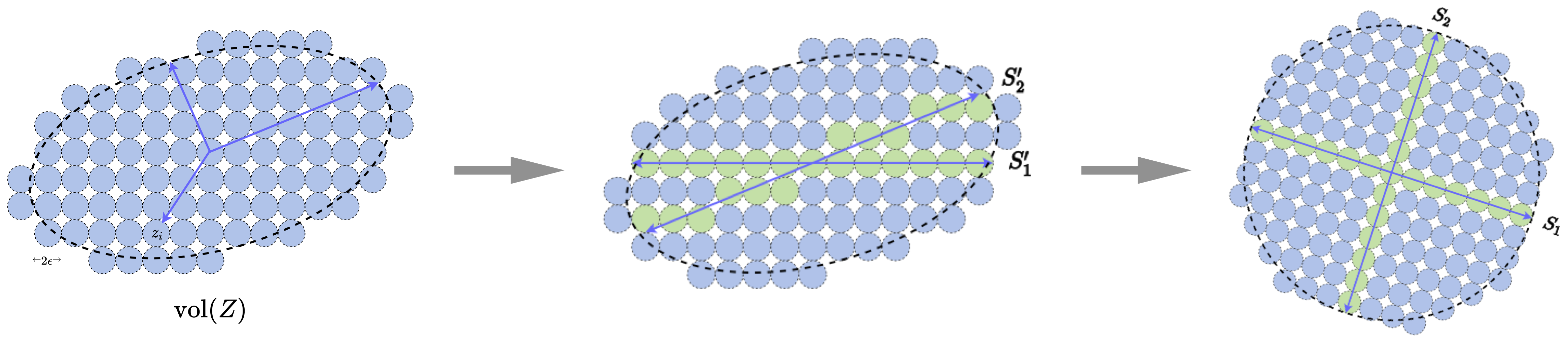
Example 4.7. Figure 4.6 shows an example in which the data \(\vX \) are distributed around two subspaces (or low-dimensional Gaussians). If they are viewed and coded together as one single Gaussian, the associated discrete (lossy) code book, represented by all the blue balls, is obviously very redundant. We can try to identify the locations of the two subspaces, denoted by \(S_1\) and \(S_2\), and design a code book that only covers the two subspaces, i.e., the green balls. If we can correctly partition samples in the data \(\vX \) into the two subspaces: \(\vX = [\vX _1, \vX _2]\bm \Pi \) with \(\vX _1 \in S_1\) and \(\vX _2 \in S_2\), where \(\bm \Pi \) denotes a permutation matrix, then the resulting coding rate for the data will be much lower. This gives a more parsimonious, hence more desirable, representation of the data. \(\blacksquare \)
So, more generally speaking, if the data are drawn from any mixture of subspaces or low-dimensional Gaussians, it would be desirable to identify those components and encode the data based on the intrinsic dimensions of those components. It turns out that we do not lose much generality by assuming that the data are drawn from a mixture of low-dimensional Gaussians. This is because a mixture of Gaussians can closely approximate most general distributions [BDS16].
The clustering problem. Now for this specific family of distributions, how can we effectively and efficiently identify those low-dimensional components from a set of samples
drawn from them? In other words, given the whole data set \(\vX \), we want to partition, or cluster, it into multiple, say \(K\), subsets:
where each subset consists of samples drawn from only one low-dimensional Gaussian or subspace and \(\bm \Pi \) is a permutation matrix to indicate membership of the partition. Note that, depending on the situation, the partition could be either deterministic or probabilistic. As shown in [MDH+07b], for a mixture of Gaussians, probabilistic partition does not lead to a lower coding rate. So for simplicity, we here consider a deterministic partition only.
Clustering via lossy compression. The main difficulty in solving the above clustering problem is that we normally do not know the number of clusters \(K\), nor do we know the dimension of each component. There has been a long history for the study of this clustering problem. The textbook [VMS16] gives a systematic and comprehensive coverage of different approaches to this problem. To find an effective approach to this problem, we first need to understand and clarify why we want to cluster. In other words, what exactly do we gain from clustering the data, compared with not to? How do we measure the gain? From the perspective of data compression, a correct clustering should lead to a more efficient encoding (and decoding) scheme.
For any given data set \(\vX \), there are already two obvious encoding schemes as the baseline. They represent two extreme ways to encode the data:
Simply view all the samples together drawn as from one single Gaussian. The associated coding rate is, as derived before, given by:
Simply memorize all the samples separately by assigning a different number to each sample. The coding rate would be:
Note that either coding scheme can become the “optimal” solution for certain (extreme) choice of the quantization error \(\epsilon \):
Note that the first scheme corresponds to the scenario when one does not care about anything interesting about the distribution at all. One does not want to spare any bit for anything informative. We call this the “lazy regime.” The second scheme corresponds to the scenario when one wants to decode every sample with an extremely high precision. So one would better “memorize” every sample. We call this the “memorization regime.”
Notice that these asymptotics in terms of \(\epsilon \) are exactly those discussed when introducing the lossy coding rate as a quantity that realistically-trained diffusion models approximate, as in the end of Section 3.3. In the current situation, we explicitly code the distribution up to precision \(\epsilon \); in the case of diffusion models, we implicitly code the distribution. Certain properties of the scheme such as memorization and generalization manifest similarly in both cases, and indeed one can study one case to understand the other.
Example 4.8. To see when the memorization regime is preferred or not, let us consider a number, say \(N\), of samples randomly distributed in a unit area on a 2D plane.14 Imagine we try to design a lossy coding scheme with a fixed quantization error \(\epsilon \). This is equivalent to putting an \(\epsilon \)-disc around each sample, as shown in Figure 4.7. When \(N\) is small, the chance that all the discs overlap with each other is zero. A codebook of size \(N\) is necessary and optimal in this case. When \(N\) or the density reaches a certain critical value \(N_c\), with high probability all the discs start to overlap and connect into one cluster that covers the whole plane—this phenomenon is known as continuum “percolation” [Gil61; MM12]. When \(N\) becomes larger than this value, the discs overlap heavily. The number \(N\) of discs becomes very redundant because we only want to encode points on the plane up to the given precision \(\epsilon \). The number of discs needed to cover all the samples is much less than \(N\).15 \(\blacksquare \)
Both the lazy and memorization regimes are somewhat trivial and perhaps are of little theoretical or practical interest. Either scheme would be far from optimal when used to encode a large number of samples drawn from a distribution that has a compact and low-dimensional support. The interesting regime exists in between these two.


Figure 4.8 shows an example with noisy samples drawn from two lines and one plane in \(\R ^3\). As we notice from the plot (c) on the right, the optimal coding rate decreases monotonically as we increase \(\epsilon \), as anticipated from the property of the rate distortion function. The plots (a) and (b) show, when varying \(\epsilon \) from very small (near zero) to very large (towards infinite), the optimal number of clusters when the coding rate is minimal. We can clearly see the lazy regime and the memorization regime on the two ends of the plots. But one can also notice in plot (b), when the quantization error \(\epsilon \) is chosen to be around the level of the true noise variance \(\epsilon _0\), the optimal number of clusters is the “correct” number three that represents two lines and one plane. We informally refer to this middle regime as the “generalization regime”. Notice that a sharp phase transition takes place between these regimes.16 \(\blacksquare \)
From the above discussion and examples, we see that, when the quantization error relative to the sample density17 is in a proper range, minimizing the lossy coding rate would allow us to uncover the underlying (low-dimensional) distribution of the sampled data. Hence, quantization, started as a choice of practicality, seems to be becoming necessary for learning a continuous distribution from its empirical distribution with finite samples. Although a rigorous theory for explaining this phenomenon remains elusive, here, for learning purposes, we care about how to exploit the phenomenon to design algorithms that can find the correct distribution.
Let us use the simple example shown in Figure 4.6 to illustrate the basic ideas. If one can partition all samples in \(\vX \) into two clusters in \(\vX _1\) and \(\vX _2\), with \(N_1\) and \(N_2\) samples respectively, then the associated coding rate would be18
where we use \(\boldsymbol {\Pi }\) to indicate membership of the partition. If the partition respects the low-dimensional structures of the distribution, in this case \(\vX _1\) and \(\vX _2\) belonging to the two subspaces respectively, then the resulting coding rate should be significantly smaller than the above two basic schemes:
In general, we can cast the clustering problem into an optimization problem that minimizes the coding rate:
Optimization strategies to cluster. The remaining question is how we optimize the above coding rate objective to find the optimal clusters. There are three natural approaches to this objective:
The first approach is not so appealing computationally as the number of possible partitions that one needs to try is exponential in the number of samples. For example, the number of partitions of \(\vX \) into two subsets of equal size is \(N \choose N/2\) which explodes as \(N\) becomes large. We will explore the third approach in the next Chapter 5. There, we will see how the role of deep neural networks, transformers in particular, is connected with the coding rate objective.
The second approach was originally suggested in the work of [MDH+07b]. It demonstrates the benefit of being able to evaluate the coding rate efficiently (say with an analytical form). With it, the (low-dimensional) clusters of the data can be found rather efficiently and effectively via the principle of minimizing coding length (MCL). Note that for a cluster \(\vX _k\) with \(N_k\) samples, the length of binary bits needed to encode all the samples in \(\vX _k\) is given by:19
If we have two clusters \(\vX _k\) and \(\vX _l\), if we want to code the samples as two separate clusters, the length of binary bits needed is
The last two terms are the number of bits needed to encode the memberships of samples according to the Huffman code.
Then, given any two separate clusters \(\vX _1\) and \(\vX _2\), we can decide whether to merge them or not based on the difference between the two coding lengths:
is positive or negative and \(\vX _k \cup \vX _l\) denotes the union of the sets of samples in \(\bm X_k\) and \(\bm X_l\). If it is positive , it means the coding length would become smaller if we merge the two clusters into one. This simple fact leads to the following clustering algorithm proposed by [MDH+07b]:
Note that this algorithm is tractable as the total number of (pairwise) comparisons and merges is about \(O(N^2\log N)\). However, due to its greedy nature, there is no theoretical guarantee that the process will converge to the globally optimal clustering solution. Nevertheless, as reported in [MDH+07b], in practice, this seemingly simple algorithm works extremely well. The clustering results plotted in Figure 4.8 were actually computed by this algorithm.
Example 4.10 (Image Segmentation). The above measure of coding length and the associated clustering algorithm assume the data distribution is a mixture of (low-dimensional) Gaussians. Although this seems somewhat idealistic, the measure and algorithm can already be very useful and even powerful in scenarios when the model is (approximately) valid.
For example, a natural image typically consists of multiple regions with nearly homogeneous textures. If we take many small windows from each region, they should resemble samples drawn from a (low-dimensional) Gaussian, as illustrated in Figure 4.9. Figure 4.10 shows the results of image segmentation based on applying the above clustering algorithm to the image patches directly. More technical details regarding customizing the algorithm to the image segmentation problem can be found in [MRY+11]. \(\blacksquare \)
So far in this chapter, we have discussed how to identify a distribution with low-dimensional structures through the principle of compression. As we have seen from the previous two sections, computational compression can be realized through either the denoising operation or clustering. Figure 4.11 illustrates this concept with our favorite example.
It is important to note that the clustering algorithm and the coding rate formulas developed in the previous section assumed that the data distribution is already (approximately) a mixture of low-dimensional Gaussians. In practice, the raw data—images, audio, text—rarely satisfy this assumption directly: their intrinsic structures are typically nonlinear. The purpose of this section is to develop a framework for transforming data so that their representations do take the form of a mixture of incoherent low-dimensional subspaces, at which point the tools from the preceding section become directly applicable. That is, the preceding section answers “how to compress and cluster data that are already Gaussian,” while this section answers “how to transform data so that they become Gaussian.” As we will see in Chapter 5, deep networks are precisely the computational mechanism for realizing such transformations, with the network’s architecture derived from optimizing the coding rate objective developed here.
Indeed, the ultimate goal for identifying a data distribution is to use it to facilitate certain subsequent tasks such as segmentation, classification, or generation (of images). Hence, how the resulting distribution is “represented” matters tremendously with respect to how information related to these subsequent tasks can be efficiently and effectively retrieved and utilized. This naturally raises a fundamental question: what makes a representation truly “good” for downstream use? In the following, we will explore the essential properties that a meaningful and useful representation should possess, and how these properties can be explicitly characterized and pursued via maximizing information gain.
How to measure the goodness of representations. One may view a given dataset as samples of a random vector \(\vx \) with a certain distribution in a high-dimensional space, say \(\R ^D\). Typically, the distribution of \(\vx \) has a much lower intrinsic dimension than the ambient space. Generally speaking, learning a representation refers to learning a continuous mapping, say \(f(\cdot )\), that transforms \(\vx \) to a so-called feature vector \(\vz \) in another (typically lower-dimensional) space, say \(\R ^d\), where \(d < D\). It is hopeful that through such a mapping
the low-dimensional intrinsic structures of \(\vx \) are identified and represented by \(\vz \) in a more compact and structured way so as to facilitate subsequent tasks such as classification or generation. The feature \(\vz \) can be viewed as a (learned) compact code for the original data \(\vx \), so the mapping \(f\) is also called an encoder. The fundamental question of representation learning is
What is a principled and effective measure for the goodness of representations?
Conceptually, the quality of a representation \(\vz \) depends on how well it identifies the most relevant and sufficient information of \(\vx \) for subsequent tasks and how efficiently it represents this information. For a long time, it was believed and argued that the “sufficiency” or “goodness” of a learned feature representation should be defined in terms of a specific task. For example, \(\vz \) just needs to be sufficient for predicting the class label \(\y \) in a classification problem. Below, let us start with the classic problem of image classification and argue why such a notion of a task-specific “representation” is limited and needs to be generalized.
Suppose that \(\bm {x} \in \R ^D\) is a random vector drawn from a mixture of \(K\) (component) distributions \(\mathcal {D} = \{\mathcal {D}_k\}_{k=1}^K\). Given a finite set of i.i.d. samples \(\vX = [\vx _1, \vx _2, \ldots , \vx _N] \in \Re ^{D\times N}\) of the random vector \(\bm x\), we seek a good representation through a continuous mapping \(f(\vx ): \R ^D \rightarrow \R ^d\) that captures intrinsic structures of \(\vx \) and best facilitates the subsequent classification task.20 To ease the task of learning distribution \(\mathcal {D}\), in the popular supervised classification setting, a true class label (or a code word for each class), usually represented by a one-hot vector \(\y _i \in \R ^K\), is given for each sample \(\vx _i\).
Encoding class information via cross entropy. Extensive studies have shown that for many practical datasets (e.g., images, audio, and natural languages), the (encoding) mapping from the data \(\bm {x}\) to its class label \(\bm {y}\) can be effectively modeled by training a deep network,21 here denoted as
with network parameters \(\theta \in \Theta \), where \(\Theta \) denotes the parameter space. For the output \(f(\vx , \theta )\) to match well with the label \(\y \), we like to minimize the cross-entropy loss over a training set \(\{(\vx _i, \y _i)\}_{i=1}^N\):22
The optimal network parameters \(\theta \) are typically found by optimizing the above objective through an efficient gradient descent scheme, with gradients computed via back propagation, as described in Section A.2.3 of Chapter A.
Despite its effectiveness and enormous popularity, there are two serious limitations with this approach: (1) It aims only to predict the labels \(\y \) even if they might be mislabeled. Empirical studies show that deep networks, used as a “black box,” can even fit random labels [ZBH+17]. (2) With such an end-to-end data fitting, despite plenty of empirical efforts in trying to interpret the so-learned features, it is not clear to what extent the intermediate features learned by the network capture the intrinsic structures of the data that make meaningful classification possible in the first place. The precise geometric and statistical properties of the learned features are also often obscured, which leads to the lack of interpretability and subsequent performance guarantees (e.g., generalizability, transferability, and robustness, etc.) in deep learning. Therefore, one of the goals of this section is to address such limitations by reformulating the objective towards learning explicitly meaningful and useful representations for the data \(\vx \), not limited to classification.
Minimal discriminative features via information bottleneck. One popular approach to interpret the role of deep networks is to view outputs of intermediate layers of the network as selecting certain latent features \(\vz = f(\vx , \theta ) \in \Re ^d\) of the data that are discriminative among multiple classes. Learned representations \(\vz \) then facilitate the subsequent classification task for predicting the class label \(\y \) by optimizing a classifier \(g(\vz )\):
We know from (4.1.13) that the mutual information between two random variables, say \(\vx ,\vz \), is defined to be
where \(H(\vx \vert \vz )\) is the conditional entropy of \(\vx \) given \(\vz \). The mutual information is also known as the information gain: It measures how much the entropy of the random variable \(\vx \) can be reduced once \(\vz \) is given. Or equivalently, it measures how much information \(\vz \) contains about \(\vx \). The information bottleneck (IB) formulation [TZ15] further hypothesizes that the role of the network is to learn \(\vz \) as the minimal sufficient statistics for predicting \(\y \). Formally, it seeks to maximize the mutual information \(I(\vz , \y )\) between \(\vz \) and \(\y \) while minimizing the mutual information \(I(\vx , \vz )\) between \(\vx \) and \(\vz \):
Given one can overcome some caveats associated with this framework [KTV18], such as how to accurately evaluate mutual information with finite samples of degenerate distributions, this framework can be helpful in explaining certain behaviors of deep networks. For example, recent work [PHD20] indeed shows that the representations learned via the cross-entropy loss (4.2.2) exhibit a neural collapse phenomenon. That is, features of each class are mapped to a one-dimensional vector whereas all other information of the class is suppressed, as illustrated in Figure 4.12.23
Remark 4.4 (Neural Collapse). Neural collapse refers to a phenomenon observed in deep neural networks trained for classification, where the learned feature representations and classifier weights exhibit highly symmetric and structured behavior during the terminal phase of training [PHD20; YWZ+22; ZDZ+21]. Specifically, within each class, features collapse to their class mean, and across classes, these means become maximally separated, forming a simplex equiangular configuration. The linear classifier aligns with the class mean up to rescaling. Additionally, the last-layer classifier converges to choosing whichever class has the nearest train class mean. Neural collapse reveals deep connections between optimization dynamics, generalization, and geometric structures arising in supervised learning.
From the above example of classification, we see that the so-learned representation \(\vz \) of \(\vx \) gives a very simple encoder that essentially maps each class of data to only one code word: the one-hot vector representing each class. From the lossy compression perspective, such an encoder is too lossy to preserve information in the data distribution. Other information, such as that useful for tasks such as image segmentation, completion, or generation, is severely lost in such a supervised learning process.
To remedy this situation, we want to learn a different encoding scheme such that the resulting feature representation \(\vz \) can capture as much information about the data distribution as possible, not limited to that useful for classification alone. More precisely, we want the representation \(\vz = f(\vx , \theta )\) to be such that there exists a decoder \(g(\vz ,\eta )\) so that:
We will formally introduce such an encoding-decoding scheme as an “autoencoder” and such a representation \(\vz \) as a “consistent” representation in Chapter 6. For now, the reader may simply view this as a generalization to the quantization code \(\hat \vx \) introduced in the preceding section for the rate distortion (in the native data \(\vx \) domain).
In the formulation of information bottleneck (4.2.5), it does not require the learned feature representation \(\vz \) to be consistent. Hence, at least it should be fixed with an objective for a (consistent) representation learning (RL):
Solving the above problem in the most general setting is a very daunting task. In general, we do not even know what classes of encoders or decoders could ensure the consistency24 Also, since we do not know the distribution of the representation \(\vz \), computing the mutual information \(I(\vz ;\y )\) can be very challenging, if not impossible.
Before we study how to approach this problem in general settings (in later Chapters), for the rest of this chapter, we will demonstrate how to solve it, in some limited way, for the special setting when the data distribution consists of clear (low-dimensional) classes.
Whether the given data \(\vX \) of a mixed distribution \(\mathcal {D}\) can be effectively classified or clustered depends on how separable (or discriminative) the component distributions \(\mathcal {D}_k\) are (or can be made). One popular working assumption is that the distribution of each class has relatively low-dimensional intrinsic structures. Hence we may assume that the distribution \(\mathcal {D}_k\) of each class has a support on a low-dimensional submanifold, say \(\mathcal {M}_k\) with dimension \(d_k \ll D\), and the distribution \(\mathcal D\) of \(\vx \) is supported on the mixture of those submanifolds, \(\mathcal M = \cup _{k=1}^K \mathcal {M}_k\), in the high-dimensional ambient space \(\Re ^D\), as illustrated before in Figure 4.1.
Not only do we need to identify the low-dimensional distribution, but we also want to represent the distribution in a form that best facilitates subsequent tasks such as classification, clustering, and conditioned generation (as we will see in the future). To do so, we require our learned feature representations to have the following properties:
We refer to such a representation the linear discriminative representation (LDR).
Notice that the first property aligns well with the objective of the classic principal component analysis (PCA) that we have discussed in Section 2.1.1. It essentially says that features of samples that belong to the same class25 should become or be made highly correlated. In other words, feature representation should be contractive for samples that are similar.
The second property requires that for samples that belong to different classes or are believed to be dissimilar, their features should be made (geometrically) incoherent or (statistically) independent, as illustrated before in Figure 4.1. Figure 4.13 illustrates when the data distribution is actually a mixture of low-dimensional submanifolds. Through compression (denoising or clustering), we first identify that the true data distribution (left). We then would like to transform the distribution so that the submanifolds eventually become mutually incoherent/independent linear subspaces (right).
Remark 4.5 (Linear Discriminative Analysis). One may notice that the second criterion resembles that of the classic linear discriminant analysis (LDA) [HTF09]. Linear discriminant analysis (LDA) [HTF09] is a supervised dimensionality reduction technique that aims to find a linear projection of data that maximizes class separability. Specifically, given labeled data, LDA seeks a linear transformation that projects high-dimensional inputs onto a lower-dimensional space where the classes are maximally separated. Note that PCA is an unsupervised method that projects data onto directions of maximum variance without considering class labels. While PCA focuses purely on preserving global variance structure, LDA explicitly exploits label information to enhance discriminative power; see the comparison in Figure 4.14.

But LDA only performs a linear projection of the original data. As we will see LDR can be more general: it seeks a, probably nonlinear, transformation to make the resulting representation linear and incoherent.
Remark 4.6 (Contrastive Learning). One may notice that the conventional contrastive learning [HCL06; HFW+19; OLV18] aims to achieve similar goals for feature representation as the first two properties stipulate. For data that belong to \(k\) different classes, a randomly chosen pair \((\vx _i, \vx _j)\) is of high probability belonging to different classes if \(k\) is large.26 Hence it is desirable that the representation \(\vz _i = f(\vx _i, \bm \theta )\) of a sample \(\vx _i\) should be highly incoherent to those \(\vz _j\) of other samples \(\vx _j\) whereas coherent to feature of its transformed version \(\tau (\vx _i)\), denoted as \(\vz (\tau (\vx _i))\) for \(\tau \) in certain augmentation set \(\mathcal T\) in consideration. Hence it was proposed heuristically that, to promote discriminativeness of the learned representation, one may seek to minimize the so-called contrastive loss:
The third property is also important because we want the learned features to reveal all possible causes of why one class is different from all other classes. For example, to tell “apple” from “orange”, we care not only about color but also shape and the leaves. Ideally, the dimension of each subspace \(\{\mathcal {S}_k\}\) should be equal to that of the corresponding submanifold \(\mathcal {M}_k\). This property will be important if we would like the map \(f(\vx ,\theta )\) to be invertible for tasks such as image generation. For example, if we draw different sample points from the feature subspace for “apple”, we should be able to decode them, via an inverse map \(g(\vz , \eta )\), to generate diverse images of apples. Such a pair of mutually inverse mappings \(f\) and \(g\) makes an autoencoding which we will study in great detail in Chapter 6. Notice that feature representations learned from minimizing the cross entropy (4.2.2) normally do not have this property, as they suffer the so-called neural collapse phenomenon discussed earlier (see Remark 4.4).
In general, although the intrinsic structures of each class/cluster may be low-dimensional, they are by no means simply linear (or Gaussian) in their original representation \(\vx \) and they need to be made linear first, through some nonlinear transformation.27 Therefore, overall, we use the nonlinear transformation \(f(\vx ,\theta )\) to seek a representation of the data such that the subspaces that represent all the classes are maximally incoherent linear subspaces. To be more precise, we want to learn a mapping \(\vz = f(\vx ,\theta )\) that maps each of the submanifolds \(\mathcal {M}_k \subset \Re ^D\) (Figure 4.13 left) to a linear subspace \(\mathcal {S}_k \subset \Re ^d\) (Figure 4.13 right). To some extent, the resulting multiple subspaces \(\{\mathcal {S}_k\}\) can be viewed as discriminative generalized principal components [VMS16] or, if orthogonal, independent components [HO00a] of the resulting features \(\vz \) for the original data \(\bm x\). As we will see in the next Chapter 5, deep networks precisely play the role of modeling and realizing this nonlinear transformation from the data distribution to linear discriminative representations.
Although the three properties—between-class discriminative, within-class compressible, and maximally diverse representation—for linear discriminative representations (LDRs) are all highly desired properties of the learned representation \(\vz \), they are by no means easy to obtain: Are these properties compatible so that we can expect to achieve them all at once? If so, is there a simple but principled objective that can measure the goodness of the resulting representations in terms of all these properties? The key to these questions is to find a principled “measure of compactness” or “information gain” for the distribution of a random variable \(\vz \) or from its finite samples \(\{\bm z_i\}_{i=1}^N\). Such a measure should directly and accurately characterize intrinsic geometric or statistical properties of the distribution, in terms of its intrinsic dimension or volume. Unlike the cross entropy (4.2.2) or information bottleneck (4.2.5), such a measure should not depend exclusively on class labels so that it can work in more general settings such as supervised, self-supervised, semi-supervised, and unsupervised settings (as we will see in later sections).
Without loss of generality, assume that the distribution \(\mathcal D\) of the random vector \(\vx \) is supported on a mixture of distributions, i.e., \(\mathcal D = \cup _{k=1}^K \mathcal {D}_k\), where each \(\mathcal {D}_k \subset \Re ^D\) has a low intrinsic dimension in the high-dimensional ambient space \(\Re ^D\). Let \(\bm X_k \in \Re ^{D\times N_k}\) denote the data matrix whose columns are samples drawn from the distribution \(\mathcal {D}_k\), where \(N_k\) denotes the number of samples for each \(k=1,\dots ,K\). Then, we use \(\bm X=[\bm X_1,\dots ,\bm X_K] \in \Re ^{D\times N}\) to denote all the samples, where \(N=\sum _{k=1}^K N_k\). Recall that we also use \(\vx _i\) to denote the \(i\)-th sample of \(\vX \), i.e., \(\vX =[\vx _1,\dots ,\vx _N] \). Under an encoding mapping:
the input samples are mapped to \(\vz _i = f(\vx _i)\) for each \(i=1,\dots ,N\). With an abuse of notation, we also write \(\vZ _k = f(\vX _k)\) and \(\vZ = f(\vX )\). Therefore, we have \(\vZ = [\bm Z_1,\dots ,\bm Z_K]\) and \(\vZ = [\vz _1,\dots \vz _N]\).
On one hand, for learned features to be discriminative, features of different classes/clusters are preferred to be maximally incoherent to each other. Hence, they together should span a space of the largest possible volume (or dimension) and the coding rate of the whole set \(\vZ \) should be as large as possible. On the other hand, learned features of the same class/cluster should be highly correlated and coherent. Hence, each class/cluster should only span a space (or subspace) of a very small volume and the coding rate should be as small as possible. Now, we will introduce how to measure the coding rate of the learned features.
Coding rate of features. Notably, a practical challenge in evaluating the coding rate is that the underlying distribution of the feature representations \(\vZ \) is typically unknown. To address this, we may approximate the features \(\vZ = [\vz _1, \ldots , \vz _N]\) as samples drawn from a multivariate Gaussian distribution. Under this assumption, as discussed in Section 4.1.3, the compactness of the features \(\vZ \) as a whole can be measured in terms of the average coding length per sample, referred to as the coding rate, subject to a precision level \(\epsilon > 0\) (see (4.1.30)) defined as follows:
On the other hand, we hope that a nonlinear transformation \(f(\vx )\) maps each class-specific submanifold \(\mathcal {M}_k \subset \R ^D\) to a maximally incoherent linear subspace \(\mathcal {S}_k \subset \R ^d\) such that the learned features \(\vZ \) lie in a union of low-dimensional subspaces. This structure allows for a more accurate evaluation of the coding rate by analyzing each subspace separately. Recall that the columns of \(\vZ _k\) denotes the features of the samples in \(\vX _k\) for each \(k=1,\dots ,K\). The coding rate for the features in \(\bm Z_k\) can be computed as follows:
Then, the sum of the average coding rates of features in each class is
Therefore, a good representation \(\vZ \) of \(\vX \) is the one that achieves a large difference between the coding rate for the whole and that for all the classes:
Notice that, as per our discussions earlier in this chapter, this difference can be interpreted as the amount of “information gained” by identifying the correct low-dimensional clusters \(\vZ _k\) within the overall set \(\vZ \).
If we choose our feature mapping \(f(\cdot )\) to be a deep neural network \(f(\cdot ,\theta )\) with network parameters \(\theta \), the overall process of the feature representation and the resulting rate reduction can be illustrated by the following diagram:
Note that \(\Delta R_{\epsilon }\) is monotonic in the scale of the features \(\vZ \). To ensure fair comparison across different representations, it is essential to normalize the scale of the learned features. This can be achieved by either imposing the Frobenius norm of each class \(\vZ _k\) to scale with the number of features in \(\vZ _k \in \mathbb R^{d \times N_k}\), i.e., \(\|\vZ _k\|_F^2 = N_k\), or by normalizing each feature to be on the unit sphere, i.e., \(\vz _i \in \mathbb {S}^{d-1}\), where \(N_k\) denotes the number of samples in the \(k\)-th class. This formulation offers a natural justification for the need for “batch normalization” in the practice of training deep neural networks [IS15].
Once the representations are comparable, the goal becomes to learn a set of features \(\vZ = f(\vX , \theta )\) such that they maximize the reduction between the coding rate of all features and that of the sum of features w.r.t. their classes:
We refer to this as the principle of maximal coding rate reduction (MCR\(^2\)), as an embodiment of Aristotle’s famous quote:
“The whole is greater than the sum of its parts.”
To learn the best representation, we require that the whole is maximally greater than the sum of its parts. To a large extent, the quantity \(\Delta R\) can be viewed as a computable realization to the mutual information term \(I(\vz ; \y )\) introduced in the objective (4.2.7).
Example 4.11. To further elucidate the ideas, let us examine the example shown in Figure 4.15.
From a compression perspective, the representation on the right is the most compact one in the sense that the difference between the coding rate when all features are encoded as a single Gaussian (blue) and that when the features are properly clustered and encoded as two separate subspaces (green) is maximal.28 \(\blacksquare \)
Note that the above MCR\(^2\) principle is designed for supervised learning problems, where the group memberships (or class labels) are known. There are a variety of ways to use the principle, or suitable generalizations, in ways which circumvent this requirement for class labels; we will discuss these later in this Chapter and in the next Chapter 5. To get a first taste, we extend the principle to unsupervised learning problems by introducing a membership matrix, which encodes the (potentially soft) assignment of each data point to latent groups or clusters. Specifically, let \(\bm \Pi = \{\bm \Pi _k\}_{k=1}^K \subset \R ^{N\times N}\) be a set of diagonal matrices whose diagonal entries encode the membership of the \(N\) samples into \(K\) classes. That is, \(\bm \Pi \) lies in a simplex \(\Omega \doteq \{\bm \Pi : \bm \Pi _k \ge \bm 0: \sum _{k=1}^K \bm \Pi _k = \bm I_N\}\). Then, we can define the average coding rate with respect to the partition \(\bm \Pi \) as
When \(\bm Z\) is given, \(R_{\epsilon }^c(\vZ \vert \bm \Pi )\) is a concave function of \(\bm \Pi \). Then the MCR\(^2\) principle for unsupervised learning problems becomes as follows:
Compared to (4.2.15), the formulation here allows for the joint optimization of both the group memberships and the network parameters. In particular, when \(\bm \Pi \) is fixed to a group membership matrix that assigns \(N\) data points into \(K\) groups, Problem (4.2.17) can recover Problem (4.2.15).
Remark 4.7 (Computing Coding Rates). It is a classical fact that computing the log-determinant of an \(n \times n\) matrix takes \(\cO (n^{3})\) time to compute. Hence computing the coding rates \(\Delta R_{\epsilon }\) or \(R_{\epsilon }\) (etc.) seem intractable at the scale of modern data analysis. There are several ways around this, which we will use without comment in the experiments that power the rest of the book.
Use the structure of the coding rate. Suppose that \(\vZ \) is an element of \(\R ^{d \times n}\). Then it holds
Use the symmetry of the Gramian. Note that \(\vZ \vZ ^{\top }\) (and similarly \(\vZ ^{\top }\vZ \)) is a symmetric matrix. Hence it is relatively cheap (though still cubic time) to compute its eigenvalues \(\lambda _{i}(\vZ \vZ ^{\top })\). Then the log-determinant can be expressed as follows:
Use the positive definiteness of the input to the log determinant. Since \(\vZ \vZ ^{\top }\) (and similarly \(\vZ ^{\top }\vZ \)) is symmetric positive semidefinite, the quantity \(\vI + \alpha \vZ \vZ ^{\top }\) is symmetric positive definite. This means we can compute the Cholesky decomposition \(\vL \vL ^{\top } = \vI + \alpha \vZ \vZ ^{\top }\), where \(\vL \in \R ^{d \times d}\) is a lower-triangular matrix with positive diagonal entries. Then
In this subsection, we study the optimization properties of the MCR\(^2\) function by analyzing its optimal solutions and the structure of its optimization landscape. To get around the technical difficulty introduced by the neural networks, we consider a simplified version of Problem (4.2.15) as follows:
In theory, the MCR\(^2\) principle (4.2.21) benefits from great generalizability and can be applied to representations \(\vZ \) of any distributions as long as the rates \(R_\epsilon \) and \(R^c_\epsilon \) for the distributions can be accurately and efficiently evaluated. The optimal representation \(\vZ ^{\ast }\) should have some interesting geometric and statistical properties. We here reveal nice properties of the optimal representation with the special case of subspaces, which have many important use cases in machine learning. When the desired representation for \(\vZ \) is multiple subspaces, the rates \(R_\epsilon \) and \(R^c_\epsilon \) in (4.2.21) are given by (4.2.10) and (4.2.12), respectively. At the maximal rate reduction, MCR\(^2\) achieves its optimal representations, denoted as \(\vZ ^{\ast } = [\vZ _1^*,\dots ,\vZ _K^*]\) with \(\rank {(\vZ _{k}^*)}\le d_k\). One can show that \(\vZ ^{\ast }\) has the following desired properties (see [YCY+20] for a formal statement and detailed proofs).
Theorem 4.2 (Characterization of Global Optimal Solutions). Suppose \(\vZ ^{\ast } = [\vZ _1^*,\dots ,\vZ _K^*]\) is a global optimal solution of Problem (4.2.21). The following statements hold:
This theorem indicates that the MCR\(^2\) principle promotes embedding of data into multiple independent subspaces (as illustrated in Figure 4.16), with features distributed isotropically in each subspace (except for possibly one dimension). Notably, this theorem also confirms that the features learned by the MCR\(^2\) principle exhibit the desired low-dimensional discriminative properties discussed in Section 4.2.2. In addition, among all such discriminative representations, it prefers the one with the highest dimensions in the ambient space. This is substantially different from the objective of information bottleneck (4.2.5).
Regularized MCR\(^2\). The above theorem characterizes properties of the global optima of the rate reduction objectives. What about other optima, such as local ones? Due to the constraints of the Frobenius norm, it is a difficult task to analyze Problem (4.2.21) from an optimization-theoretic perspective. Therefore, we consider the Lagrangian formulation of (4.2.21). This can be viewed as a tight relaxation or even an equivalent problem of (4.2.21) whose optimal solutions agree under specific settings of the regularization parameter; see [WLP+24, Proposition 3.2]. Specifically, the formulation we study, referred to henceforth as the regularized MCR\(^2\) problem, is as follows:
where \(\lambda > 0\) is the regularization parameter. Although the program (4.2.22) is highly nonconcave and involves matrix inverses in its gradient computation, we can still explicitly characterize its local and global optima as follows (see [WLP+24, Theorem 3.1] for detailed proofs).
Theorem 4.3 (Local and Global Optima). Let \(N_k\) denote the number of training samples in the \(k\)-th class for each \(k \in \{1,\dots ,K\}\), \(N_{\max } \doteq \max \{N_1,\dots ,N_K\}\), \(\alpha =d/(N\epsilon ^2)\), and \(\alpha _{k} = d/(N_k\epsilon ^2)\) for each \(k \in \{1,\dots ,K\}\). Given a coding precision \(\epsilon > 0\), if the regularization parameter satisfies
then the following statements hold:
(i) (Local maximizers) \(\bm Z^* = \left [\bm Z_1^*,\dots ,\bm Z_K^* \right ]\) is a local maximizer of Problem (4.2.22) if and only if the
\(k\)-th block admits the following decomposition
where (a) \(r_k = \mathrm {rank}(\bm Z_k^*)\) satisfies \(r_k \in [0,\min \{N_k,d\})\) and \(\sum _{k=1}^K r_k \le \min \{N,d\}\), (b) \(\bm U_k \in \mathcal {O}^{d \times r_k}\) satisfies \(\bm U_k^{\top }\bm U_l = \bm 0\) for all \(k \neq l\), \(\bm V_k \in \mathcal {O}^{N_k \times r_k}\), and (c) \(\eta _k := (\alpha _k-\alpha ) - \lambda (N/N_k+1)\) for each \(k\in \{1,\dots ,K\}\).
(ii) (Global maximizers) \(\bm Z^* = \left [\bm Z_1^*,\dots ,\bm Z_K^* \right ]\) is a global maximizer of Problem (4.2.22) if and only if
(a) it satisfies all the above conditions and \(\sum _{k=1}^K r_k = \min \{N,d\}\), and (b) for all \(k \neq l \in [K]\) satisfying \(N_k < N_l\) and \(r_l > 0\), we have
\(r_k = \min \{N_k,d\}\).
This theorem explicitly characterizes the local and global optima of problem (4.2.22). Intuitively, this shows that the features represented by each local maximizer of Problem (4.2.22) are low-dimensional and discriminative. Although we have characterized the local and global optimal solutions in Theorem 4.3, it remains unknown whether these solutions can be efficiently computed using GD to solve the problem (4.2.22), since GD may get stuck at other critical points such as a saddle point. Fortunately, [LSJ+16; SQW15] showed that if a function is twice continuously differentiable and satisfies the strict saddle property, i.e., each critical point is either a local maximizer or a strict saddle point29, GD converges to a local maximizer almost surely with random initialization. We investigate the global optimization landscape of the problem (4.2.22) by characterizing all its critical points as follows (see [WLP+24, Theorem 3.3] for detailed proofs).
Theorem 4.4 (Benign Global Optimization Landscape). Given a coding precision \(\epsilon > 0\), if the regularization parameter satisfies (4.2.23), it holds that any critical point \(\bm Z\) of the problem (4.2.22) is either a local maximizer or a strict saddle point.
Together, the above two theorems show that the learned features associated with each local maximizer of the rate reduction objective — not just global maximizers — are structured as incoherent low-dimensional subspaces. Furthermore, the (regularized) rate reduction objective (4.2.15) has a very benign landscape with only local maxima and strict saddles as critical points, as illustrated in Figure 4.17. According to [LSJ+16; SQW15], Theorems 4.3 and 4.4 imply that low-dimensional and discriminative representations (LDRs) can be efficiently found by applying (stochastic) gradient descent to the rate reduction objective (4.2.15) from random initialization. These results also indirectly explain why in Section 4.3.1, if the chosen network is expressive enough and trained well, the resulting representation typically gives an incoherent linear representation that likely corresponds to the globally optimal solution. Interested readers are referred to [WLP+24] for proofs.
We here present how the MCR\(^2\) objective (4.2.15) helps learn better representations than the cross entropy (CE) (4.2.2) for image classification. Here, for simplicity,30 we adopt the popular neural network architecture, the ResNet-18 [HZR+16b], to model the feature mapping \(\vz = f(\vx ,\theta )\). We optimize the neural network parameters \(\theta \) via the backpropagation algorithm (detailed in Section A.2.3) to maximize the coding rate reduction. More implementation details of this experiment can be found in [CYY+22].
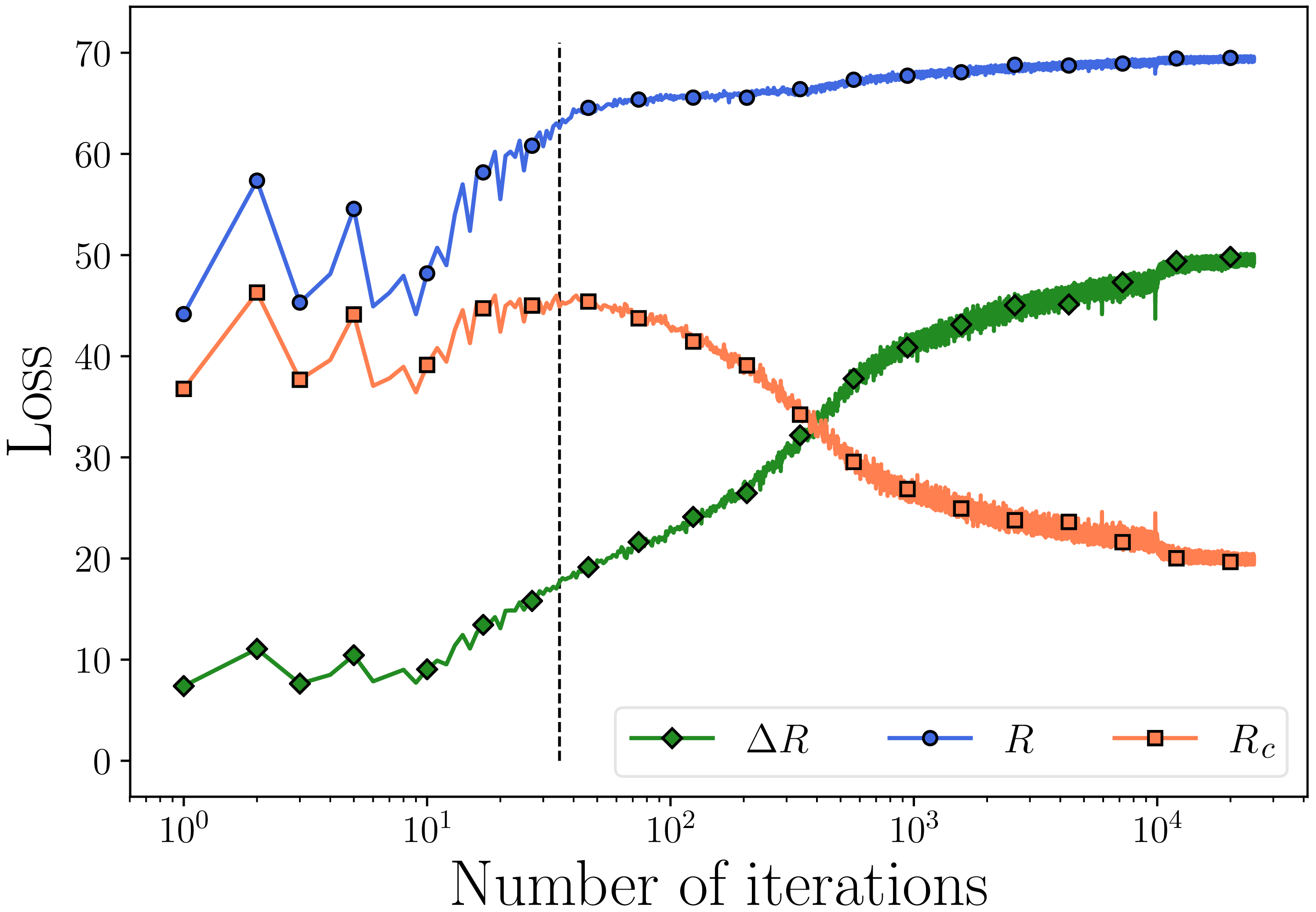
Figure 4.18 illustrates how the two rates and their difference (for both training and test data) evolve over epochs of training: After an initial phase, \(R_\epsilon \) gradually increases while \(R^c_\epsilon \) decreases, indicating that features \(\bm Z\) are expanding as a whole while each class \(\bm Z_k\) is being compressed.
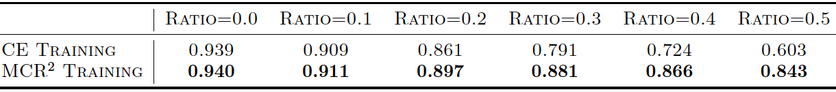
We first evaluate the performance with the CIFAR-10 image classification dataset [KH+09] and the results are shown in the table of Figure 4.19. As we can see, the MCR\(^2\) objective achieves a comparable performance as the cross entropy (CE) loss. In addition, the MCR\(^2\) objective is more robust to corruptions in the class labels since it learns a joint (subspace) representation for each class instead of trying to fit the labels of individual samples.
Figure 4.20 shows the distribution of singular values of the learned features \(\vZ _k\) per class. From the distribution of the singular values shown in Figure 4.19a, we see that the features \(\vz \) learned from MCR\(^2\) for each class are distributed on a subspace of dimension around 10-12, whereas the features from cross entropy Figure 4.19b are of much lower dimension.31
Figure 4.21 shows the cosine similarities between the learned features sorted by class. We also compare the similarities of the learned features by using the cross-entropy (CE) (4.2.2) and the MCR\(^2\) objective (4.2.15). From the plots, one can clearly see that the features learned by the MCR\(^2\) objective for different classes are much more incoherent (or independent) than features learned by using cross-entropy loss. Within each class, the features also are less coherent hence more diverse, as indicated by the distribution of their singular values shown in Figure 4.19a.
We visualize the images that are mapped along different singular vectors in the feature subspace of each class, which we call the “principal” images. Figure 4.22 shows these principal images along each of the top-10 singular vectors. As we can see, the images along each singular vector are very similar in their appearances and structures and images along different singular vectors are very distinct from each other.
Despite the fact that the MCR\(^2\) objective seems to allow us to learn better representations, there has been an apparent lack of justification of the network architectures used in the above experiments. It is yet unclear why the network adopted here (the ResNet-18) is suitable for representing the map \(f(\vx , \theta )\), let alone for interpreting the layer operators and parameters \(\theta \) learned inside. In Chapter 5, we will show how to derive network architectures and components entirely as a “white box” from the desired objective (say the rate reduction).
As we have seen in the above section, the class information makes learning a structured representation of the (mixed) data distribution relatively easy. However, such information is often not available, at least not at a massive scale.
Now we present how to extend the MCR\(^2\) principle to the unsupervised setting. Contrary to supervised learning where the class labels are known, in unsupervised learning, the group memberships of the data samples are unknown. In this case, we can apply certain class of augmentations or transformations, say \(\tau \) with a distribution \(P_{\tau }\), to each sample. For example, for images, augmentations typically include translations, rotations, or cropping of each image sample. We may view the augmented samples of each data point as belonging to the same group or cluster.
More specifically, given a set of \(N\) data samples \(\vX = [\vx _1,\dots ,\vx _N]\), we generate \(m\) augmented views \(\{\tau _i\}_{i=1}^m\) for each data point \(\vx _k\) , denoted as \(\tilde {\vX }_{k} = [\tau _1(\vx _k), \tau _2(\vx _k), \dots , \tau _m(\vx _k)]\). We treat the augmented samples \(\tilde {\vX }_{i}\) as the \(i\)-th class with \(K=N\) groups/clusters in total. Now, we can apply the MCR\(^2\) principle as we did before in the supervised learning case. Specifically, we learn the feature mapping \(f(\vx ,\theta )\) by maximizing the coding rate reduction as follows:
Here, \(\tilde {\vX } = [\tilde {\vX }_1,\dots ,\tilde {\vX }_N]\) and \(\vZ _k = f(\tilde {\vX }_k,\theta )\) denotes the features of the augmented samples of \(\vx _k\) for each \(k=1,\dots ,N\).
Let us again adopt ResNet-18 as the feature mapping \(f(\vx ,\theta )\) and optimize the network parameters \(\theta \) to maximize the unsupervised objective (4.3.1). After training on the CIFAR-10 dataset, we visualize the evolution of the two rates and their difference (for both training and test data) over epochs of training in Figure 4.22a. Similar to the supervised learning case, after an initial phase, \(R_\epsilon \) gradually increases while \(R^c_\epsilon \) decreases, indicating that features \(\bm Z\) are expanding as a whole while each cluster \(\bm Z_k\) is being compressed. Compared to the supervised case shown in Figure 4.18, we can observe that, in the unsupervised case, the total coding rate \(R_\epsilon \) expands rapidly and the overall MCR\(^2\) objective saturates at a local optimum. To alleviate this, we can alter the optimization strategy by controlling the dynamics of \(R_\epsilon \) and \(R^c_\epsilon \). Specifically, we can rescale the rates by replacing the coding rate \(R_\epsilon (\vZ )\) in (4.3.1) with
By setting \(\gamma _1 = \gamma _2 = N\), we arrive at a modified learning objective, referred to as MCR\(^2\)-CTRL, whose training dynamics are shown in Figure 4.22b. As we can see, with this controlled MCR\(^2\) objective, features are first compressed and then gradually expanded, leading to a higher value of the overall objective \(\Delta R_{\epsilon }(\vZ )\).
To assess the quality of the learned representations and verify whether they have good subspace structures, we adopt a subspace clustering algorithm EnSC [YLR+16]. For evaluation metrics, we consider normalized mutual information (NMI), clustering accuracy (ACC), and adjusted rand index (ARI) 32. For comparison, we consider methods including JULE [YPB16], RTM [NMM19], DEC [XGF16], DAC [CWM+17], and DCCM [WLW+19]. The clustering results are summarized in Figure 4.24. As we can see, the features learned by maximizing the MCR\(^2\)-CTRL objective achieve better clustering accuracy than those learned by other algorithms.
There is one main drawback though: the MCR\(^2\)-based unsupervised learning method requires a costly \(\log \det \) operation of \(\O (d^3)\) complexity per sample when computing \(R^c_\epsilon \). This quickly becomes computationally prohibitive as we try to scale to larger datasets. Instead of minimizing the exact coding rate for each group of augmented samples \(\tilde {\vX }_{i}\), we can approximate the effect of compressing features in each group by maximizing the cosine similarity between the features of the augmented samples:33
where \(\gamma > 0\) is a hyperparameter that controls the strength of the cosine similarity term, as it differs from the coding rate in magnitude. This objective avoids the costly \(\log \det \) operation and is much more scalable. In fact, this objective is closely related to popular (unsupervised) contrastive learning methods such as SimCLR [CKN+20] and DINO [CTM+21], which have been engineered to learn high-quality representations from massive amount of images.
As we will show later in Section 8.2.2 of Chapter 8, this objective (4.3.2) can be implemented very efficiently to learn a highly structured representation \(\vZ \) that is highly linear and discriminative. The learned feature representation leads to state-of-the-art performance on large real-world datasets comparable or even better than features learned by DINO, but without the heavy engineering efforts needed for DINO. Hence, we refer to this objective as Simplified DINO (SimDINO). As a preview, Table 4.1 show that SimDINO outperforms DINO on ImageNet-1k classification using both \(k\)-nearest neighbor accuracy and linear probing (i.e. training a linear classifier on pretrained models). This demonstrates that the objective leads to highly structured and linearized representations. We can also utilize these representations for downstream tasks such as unsupervised segmentation34, as illustrated in Figure 4.25. More implementation details and experimental results of SimDINO will be presented in Chapter 8.
| Method | Model | Epochs | 20-NN | Linear Probing |
| DINO | ViT-B | 100 | 72.9 | 76.3 |
| SimDINO | ViT-B | 100 | 74.9 | 77.3 |
| DINO | ViT-L | 100 | – | – |
| SimDINO | ViT-L | 100 | 75.6 | 77.4 |
Key messages. In this Chapter, we have studied basic concepts and ideas behind how to learn a distribution from finite samples and obtain a computable encoding and decoding scheme for the distribution. For distributions that are continuous and possibly low-dimensional, we have argued that such a scheme is necessarily lossy – hence the importance of the concept of rate distortion. The noise introduced through distortion, due to quantization, plays a related but different role from the noise we have studied in the preceding chapter. One may think of the noise considered in Chapter 3 as “outside” of the submanifold of the support of the distribution whereas the noise considered in this chapter is “inside” the support. Informally, we may refer to the diffusion/denoising process outside of the support as “continuation” and the diffusion/denoising process inside the support as “percolation.” A more unified analysis and understanding of their compounded effect is due for future study.
In this chapter, we introduced for the first time the concept of learning a representation for a distribution. We have considered arguably the simplest case, the case of classification. If one views the classification label \(\y \) as a fixed simple (grossly lossy) code for the data \(\vx \), we may seek a consistent35 representation \(\vz = f(\vx )\) of the data \(\vx \) such that it tends to maximize the mutual information between the representation and this simple code:
In addition, we require such a representation \(\vz \) is not only consistent to \(\vx \) but also much more structured than the native data distribution of \(\vx \) – classes are linearly discriminative. This would make the learned representation much more efficient to use than the native data distribution for subsequent tasks such as recognition, segmentation and completion. The maximal coding rate reduction objective introduced is a natural and computable realization of these requirements. In Chapter 7, we will see how to generalize this objective to a much broader context when \(\y \) could be a more general lossy code (say image caption) or a random variable related to \(\vx \).
Exercise 4.1. Please show the following properties of the \(\log \det (\cdot )\) function.
is a concave function. (Hint: The function \(f(\vx )\) is concave if and only if the one-dimensional function \(f(\vx +t\vh )\) is concave for all \(\vx \) and \(\vh \).)
where \(\lambda _1,\lambda _2,\dots ,\lambda _n\) are the eigenvalues of \(\vA \).
for a positive definite matrix \(\vA \).
Exercise 4.2. Let \(\bm Z = [\bm Z_1, \dots , \bm Z_K] \in \mathbb {R}^{d \times N}\), where each \(\bm Z_k \in \mathbb {R}^{d \times N_k}\) and \(N = \sum _{k=1}^K N_k\).
where \(\alpha > 0\).
Exercise 4.3. Let \(\vz _1\) and \(\vz _2\) be two vectors of unit length. Let \(\vZ = [\vz _1, \vz _2]\) Show that the following three objectives are equivalent:
However, they may no longer be exactly equivalent when there are more than two vectors in a high-dimensional space. The \(\log \det \) is more general as it measures the total volume spanned by all the vectors in the high-dimensional space.
Exercise 4.4. Please derive the rate-distortion function for the Gaussian random vector introduced in Example 4.4.