“Mathematics is the art of giving the same name to different things.”
\(~\) — Henri Poincaré
In the previous Chapters of this book, we have studied how to effectively and efficiently learn a representation for a variable \(\x \) in the world with a distribution \(p(\x )\) that has a low-dimensional support in a high-dimensional space. So far, we have mainly developed the methodology for learning representation and autoencoding in a general, distribution or task-agnostic fashion. With such a learned representation, one can already use it to perform some generic and basic tasks such as classification (if the encoding is supervised with the class) and generation of random samples that have the same distribution as the given data (say natural images or natural languages).
More generally, however, the universality and scalability of the theoretical and computational framework presented in this book has enabled us to learn the distribution of a variety of important real-world high-dimensional data such as natural languages, human poses, natural images, videos, and even 3D scenes. Once the intrinsically rich and low-dimensional structures of these real data can be learned and represented correctly, they start to enable a broad family of powerful, often seemingly miraculous, tasks. Hence, from here onwards, we will start to show how to connect and tailor the general methods presented in previous Chapters to learn useful representations for specific structured data distributions and for many popular tasks in modern practice of machine intelligence.
Leveraging low-dimensionality for stable and robust inference. Generally speaking, a good representation or autoencoding should enable us to utilize the learned low-dimensional distribution of the data \(\x \) and its representation \(\z \) for various subsequent classification, estimation, and generation tasks under different conditions. As we have alluded to earlier in Chapter 1 Section 1.2.2, the importance of the low-dimensionality of the distribution is the key for us to conduct stable and robust inference related to the data \(\x \), as illustrated by the few simple examples in Figure 1.11, from incomplete, noisy, and even corrupted observations. As it turns out, the very same concept carries over to real-world high-dimensional data whose distributions have a low-dimensional support, such as natural images and languages.
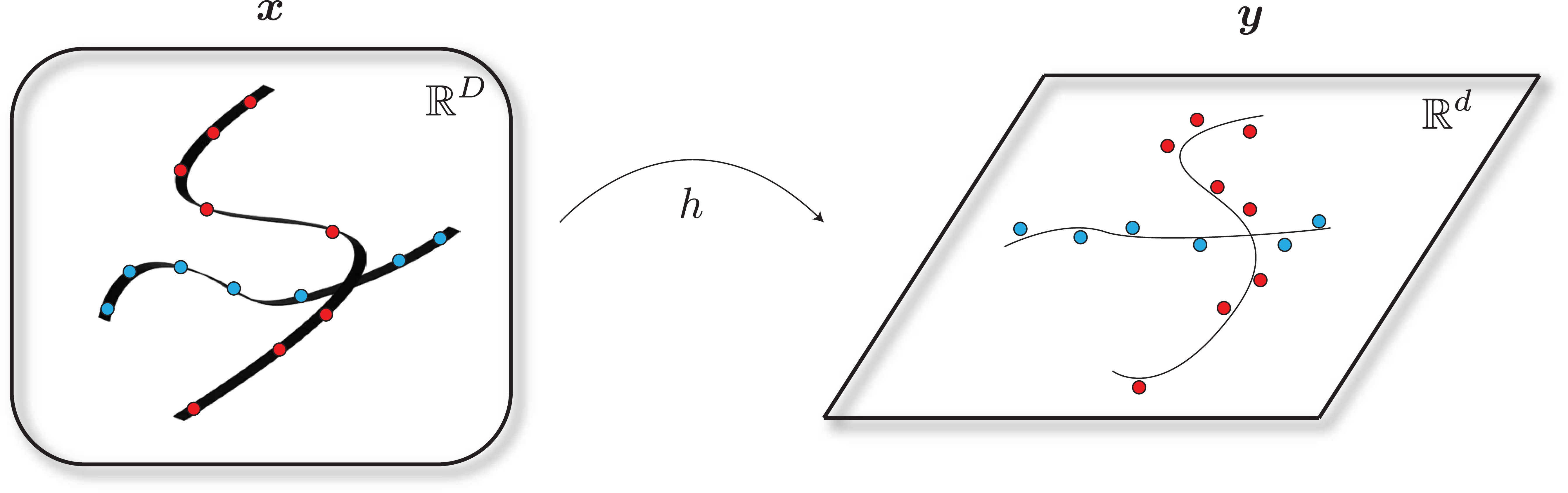
Despite a dazzling variety of applications in the practice of machine learning with data such as languages, images, videos and many other modalities, almost all practical applications can be viewed as a special case of the following inference problem: given an observation \(\y \) that depends on \(\x \), say
where \(h(\cdot )\) represents measurements of a part of \(\x \) or certain observed attributes and \(\vw \) represents some measurement noise and even (sparse) corruptions, solve the “inverse problem” of obtaining a most likely estimate \(\hat \x (\y )\) of \(\x \) or generating a sample \(\hat {\x }\) that is at least consistent with the observation \(\y \approx h(\hat {\x })\). Figure 7.1 illustrates the general relationship between \(\x \) and \(\y \).
Example 7.1 (Image Completion and Text Prediction). The popular natural image completion and natural language prediction are two typical tasks that require us to recover a full data \(\x \) from its partial observations \(\y \), with parts of \(\x \) masked out and to be completed based on the rest. Figure 7.2 shows some examples of such tasks. In fact, it is precisely these tasks which have inspired how to train modern large models for text generation (such as GPT) and image completion (such as the masked autoencoder) that we will study in greater detail later.


Statistical interpretation via Bayes’ rule. Generally speaking, to accomplish such tasks well, we need to get ahold of the conditional distribution \(p(\x \mid \y )\). If we had this, then we would be able to find the maximal likelihood estimate (prediction):
or compute the conditional expectation estimate:
or sample from the conditional distribution:
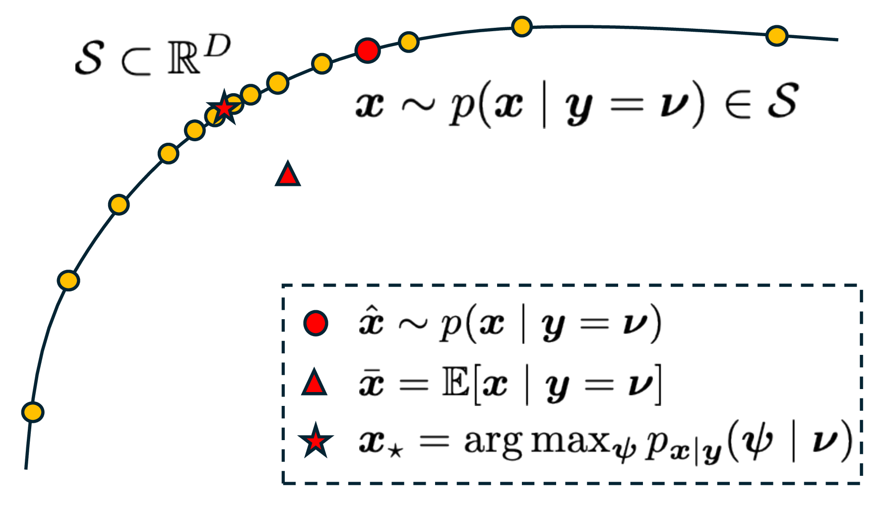
Notice that if the conditional distribution \(p(\x \mid \y )\) has a low-dimensional support that is nonlinear, these three different estimates can be rather different, as illustrated in Figure 7.3. Conceptually, the maximum a posteriori (MAP) estimate is the most desired one—it is the sample of the highest probability to have produced the observation \(\y \), but it is typically the most expensive to compute.
Notice that from Bayes’ rule, we have
For instance, the maximal likelihood estimate can be computed by solving the following (maximal log likelihood) program:
Efficiently computing the conditional distribution \(p(\x \mid \y )\) naturally depends on how we learn and exploit the low-dimensional distribution \(p(\x )\) of the data \(\x \) and the observation model \(\y = h(\x ) + \vw \) that determines the conditional distribution \(p(\y \mid \x )\).
Remark 7.1 (End-to-End versus Bayesian Inference). In the modern practice of data-driven machine learning, for certain popular tasks people often directly learn the conditional distribution \(p(\x \mid \y )\) or a (probabilistic) mapping or a regressor. Such a mapping is often modeled by some deep networks and trained end-to-end with sufficient paired samples \((\x , \y )\). Such an approach is very different from the above Bayesian approach in which both the distribution of \(\x \sim p(\x )\) and the (observation) mapping are needed. The benefit of the Bayesian approach is that the learned distribution \(p(\x )\) can facilitate many different tasks with varied observation models and conditions.
Geometric interpretation as constrained optimization. As the support \(\cS _{\vx }\) of the distribution of \(\vx \) is low-dimensional, we may assume that there exists a function \(F\) such that
such that \(\cS _{\vx } = F^{-1}(\{0\})\) is the low-dimensional support of the distribution \(p(\x )\). Geometrically, one natural choice of \(F(\x )\) is the “distance function” to the support \(\mathcal {S}_{\x }\):
Notice that, in reality, we only have discrete samples on the support of the distribution. In the same spirit of continuation, through diffusion or lossy coding studied in Chapters 3 and 4, we may approximate the distance function as \(F(\x ) \approx \min _{\x _p \in \cC _{\vx }^{\epsilon }} \|\x - \x _p\|_2\) where \(\mathcal {S}_{\x }\) is replaced by a covering \(\cC _{\vx }^{\epsilon }\) of the samples with \(\epsilon \)-balls. But if the analytical form of a simple distribution is given, sometimes \(F(\x )\) can be computed explicitly.
Example 7.2 (Distance to a Line in \(\mathbb {R}^3\)). Let us assume that the support of a low-dimensional distribution in \(\mathbb {R}^3\) is the \(x_3\)-axis. Then the distance function \(F(\x )\) is given by:
To see how such a function plays an important role in exploiting the distribution, for simplicity, we will assume that, for the rest of the subsection, the distance function is already given.
Now given \(\y = h(\x ) +\vw \), to solve for \(\x \), we can solve the following constrained optimization problem:
Using the method of augmented Lagrange multipliers, we can solve the following unconstrained program:
for some constant Lagrange multiplier \(\lambda \). This is equivalent to the following program:
where \(c \doteq {\lambda }/{\mu }\) can be viewed as a “mean” for the constraint function. As \(\mu \) becomes large when enforcing the constraint via continuation1, \(c\) becomes increasingly small. The above program may be interpreted in two different ways.
Firstly, one may view the first term as the conditional probability of \(\y \) given \(\x \), and the second term as a probability density for \(\x \):
Hence, solving the constrained optimization for the inverse problem is equivalent to conducting Bayes inference with the above probability densities. Hence solving the above program (7.1.13) via gradient ascent is equivalent to the above maximal likelihood estimate (7.1.7), in which the gradient takes the form:
where \(\pdv {h}{\vx }(\vx )\) and \(\pdv {F}{\vx }(\vx )\) are the Jacobian of \(h(\x )\) and \(F(\x )\), respectively.
Example 7.3 (Gradient of \(F(\x )\)). For the distance function defined in Example 7.2, its gradient is given by
Notice that the above (gradient)
always points towards the low-dimensional support of the distribution. Hence the descent process can be viewed as a “denoising” process, studied in Chapter 3, that gradually enforces the data to be closer to the correct support. Notice that the above derivation suggests that the “step size” of the score \(\nabla _{\x } \log p(\x )\) of the denoising process is
which for any fixed \(\mu \) is nearly proportional to the distance of the point \(\x \) to the support.
Secondly, notice that solving the above program (7.1.13) with \(\mu \) increasing is equivalent to:
Due to the conspicuous quadratic form of the two terms in the above equation, they can also be interpreted as certain “energy” functions. Such a formulation is often referred to as “Energy Minimization” in the machine learning literature, advocated by people like Yann LeCun [LCH+06]. Here the energy of a point \(\x \) is a quadratic function of its distance to the support of the desired distribution. Notice that in Chapter 3 and Chapter 4, we have argued that the notion of entropy is to measure the “volume” or uncertainty of the data distribution whereas here the energy depends on the “distance” of \(\x \) to the support of the distribution. As we minimize the above energy functions, the entropy (or uncertainty) of the feasible solutions reduces until it reaches (a feasible solution of) the optimal MAP estimate, as illustrated in Figure 7.4.
Notice that the above discussion and derivation are based on the assumption that we have perfect knowledge about the function \(F(\x )\) and the observation model \(h(\x )\). In practice, however, they may not be available at all and need to be “learned” from the data given. Hence to make the above conceptual solution truly computable, we need to deal with various situations in which information about the distributions of \(\x \) and the relationship between \(\x \) and \(\y \) are given or accessible in different ways and forms.
In general, they can mostly be categorized into four cases, which are, conceptually, increasingly more challenging:
In this chapter, we will discuss general approaches to learn the desired distributions and solve the associated conditional estimation or generation for these cases, typically with a representative practical problem. Throughout the chapter, the reader should keep Figure 7.1 in mind.
Notice that in the setting we have discussed in previous Chapters, the autoencoding network is trained to reconstruct a set of samples of the random vector \(\x \). This would allow us to regenerate samples from the learned (low-dimensional) distribution. In practice, the low-dimensionality of the distribution, once given or learned, can be exploited for stable and robust recovery, completion, or prediction tasks. That is, under rather mild conditions, one can recover \(\x \) from highly compressive, partial, noisy or even corrupted measures of \(\x \) of the kind:
where \(\y \) is typically an observation of \(\x \) that is of much lower dimension than \(\x \) and \(\vw \) can be random noise or even sparse gross corruptions. This is a class of problems that have been extensively studied in the classical signal processing literature, for low-dimensional structures such as sparse vectors, low-rank matrices, and beyond. Interested readers may see [WM22] for a complete exposition of this topic.
Here to put the classic work in a more general modern setting, we illustrate the basic idea and facts through the arguably simplest task of data (and particularly image) completion. That is, we consider the problem of recovering a sample \(\x \) when parts of it are missing (or even corrupted). We want to recover or predict the rest of \(\x \) from observing only a fraction of it:
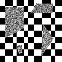
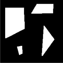
where \(\mathcal {P}_{\Omega }(\spcdot )\) represents a masking operation (see Figure 7.5 for an example).
In this section and the next, we will study the completion task under two different scenarios: One is when the distribution of the data \(\x \) of interest is already given a priori, even in a certain analytical form. This is the case that prevails in classic signal processing where the structures of the signals are assumed to be known, for example, band-limited, sparse or low-rank. The other is when only raw samples of \(\x \) are available and we need to learn the low-dimensional distribution from the samples in order to solve the completion task well. This is the case for the tasks of natural image completion or video frame prediction. As a precursor to the rest of the chapter, we start with the simplest case of image completion: when the image to be completed can be well modeled as a low-rank matrix. We will move on to increasingly more general cases and more challenging settings later.
Low-rank matrix completion. The low-rank matrix completion problem is a classical problem for data completion when its distribution is low-dimensional and known. Consider a random sample of a matrix \(\X _o = [\x _1, \ldots , \x _n] \in \mathbb {R}^{m\times n}\) from the space of all matrices of rank \(r\). In general, we assume the rank of the matrix is
So it is clear that locally the intrinsic dimension of the space of all matrices of rank \(r\) is much lower than the ambient space \(mn\).
Now, let \(\Omega \) indicate a set of indices of observed entries of the matrix \(\X _o\). Let the observed entries be:
The remaining entries supported on \(\Omega ^c\) are unobserved or missing. The problem is whether we can recover from \(\Y \) the missing entries of \(\X \) correctly and efficiently. Figure 7.5 shows one example of completing such a matrix.
Notice that the fundamental reason why such a matrix can be completed is that columns and rows of the matrix are highly correlated and they all lie on a low-dimensional subspace. For the example shown in Figure 7.5, the dimension or the rank of the matrix completed is only two. Hence the fundamental idea to recover such a matrix is to seek a matrix that has the lowest rank among all matrices that have entries agreeing with the observed ones:
This is known as the low-rank matrix completion problem. See [WM22] for a full characterization of the space of all low-rank matrices. As the rank function is discontinuous and rank minimization is in general an NP-hard problem, we would like to relax it with something easier to optimize.
Based on our knowledge about compression from Chapter 3, we could promote the low-rankness of the recovered matrix \(\X \) by enforcing the lossy coding rate (or the volume spanned by \(\X \)) of the data in \(\X \) to be small:
The problem can be viewed as a continuous relaxation of the above low-rank matrix completion problem (7.2.5) and it can be solved via gradient descent. One can show that the gradient descent operator for the \(\log \det \) objective is precisely minimizing a close surrogate of the rank of the matrix \(\X \X ^\top \).
The rate distortion function is a nonconvex function, and its gradient descent does not always guarantee finding the globally optimal solution. Nevertheless, since the underlying structure sought for \(\X \) is piecewise linear, the rank function admits a rather effective convex relaxation: the nuclear norm—the sum of all singular values of the matrix \(\X \). As shown in the compressive sensing literature, under fairly broad conditions,3 the matrix completion problem (7.2.5) can be effectively solved by the following convex program:
where the nuclear norm \(\|\X \|_*\) is the sum of singular values of \(\X \). In practice, we often convert the above constrained convex optimization program to an unconstrained one:
for some properly chosen \(\lambda > 0\). Interested readers may refer to [WM22] for how to develop algorithms that can solve the above programs efficiently and effectively. Figure 7.5 shows a real example in which the matrix \(\hat \X \) is actually recovered by solving the above program.
Further extensions. It has been shown that images (or more accurately textures) and 3D scenes with low-rank structures can be very effectively completed via solving optimization programs of the above kind, even if there is additional corruption and distortion [LRZ+12; YZB+23; ZLG+10]:
where \(\tau \) is some unknown nonlinear distortion of the image and \(\boldsymbol {E}\) is an unknown matrix that models some (sparse) occlusion and corruption. Again, interested readers may refer to [WM22] for a more detailed account.
In the previous subsection, the reason we can infer \(\x \) from the partial observation \(\y \) is because (the support of) the distribution of \(\X \) is known or specified a priori, say as the set of all low-rank matrices. For many practical datasets, we do not have their distribution in an analytical form like the low-rank matrices, say the set of all natural images. Nevertheless, if we have sufficient samples of the data \(\x \), we should be able to learn its low-dimensional distribution first and leverage it for future inference tasks based on an observation \(\y = h(\x ) + \vw \). In this section, we assume the observation model \(h(\cdot )\) is given and known. We will study the case when \(h(\cdot )\) is not explicitly given in the next section.
For a general image \(\vX \) such as the one shown on the left of Figure 7.6, we can no longer view it as a low-rank matrix. However, humans still demonstrate remarkable ability to complete a scene and recognize familiar objects despite severe occlusion. This suggests that our brain has learned the low-dimensional distribution of natural images and can use it for completion, and hence recognition. However, the distribution of all natural images is not as simple as a low-dimensional linear subspace. Hence a natural question is whether we can learn the more sophisticated distribution of natural images and use it to perform image completion?
One empirical approach to the image completion task is to find an encoding and decoding scheme by solving the following masked autoencoding (MAE) program that minimizes the reconstruction loss:
Unlike the matrix completion problem which has a simple underlying structure, we should no longer expect that the encoding and decoding mappings admit simple closed forms or the program can be solved by explicit algorithms.
For a general natural image, we can no longer assume that its columns or rows are sampled from a low-dimensional subspace or a low-rank Gaussian. However, it is reasonable to assume that the image consists of multiple regions. Image patches in each region are similar and can be modeled as one (low-rank) Gaussian or subspace. Hence, to exploit the low-dimensionality of the distribution, the objective of the encoder \(f\) is to transform \(\X \) to a representation \(\Z \):
such that the distribution of \(\Z \) can be well modeled as a mixture of subspaces, say \(\{\vU _{[K]}\}\), such that the rate reduction is maximized while the sparsity is minimized:
where the functions \(R_\epsilon (\cdot )\) and \(R^c_\epsilon (\cdot )\) are defined in (5.2.2) and (5.2.3), respectively.
As we have shown in the previous Chapter 5, the encoder \(f\) that minimizes the above objective can be constructed as a sequence of transformer-like operators. As shown in the work of [PBW+24], the decoder \(g\) can be viewed and hence constructed explicitly as the inverse process of the encoder \(f\). Figure 7.7 illustrates the overall architectures of both the encoder and the corresponding decoder at each layer. The parameters of the encoder \(f\) and decoder \(g\) can be learned by optimizing the reconstruction loss (7.3.1) via gradient descent.
Figure 7.8 shows some representative results of the thus-designed masked auto-encoder. More implementation details and results of the masked autoencoder for natural image completion can be found in Chapter 8 Section 8.5.
The above (masked) autoencoding problem aims to generate a sample image that is consistent with certain observations or conditions. But let us examine the approach more closely: given the visual part of an image \(\X _v = \mathcal {P}_{\Omega }(\X )\), we try to estimate the masked part \(\X _m = \mathcal {P}_{\Omega ^c}(\X )\). For realizations \((\vXi _v, \vXi _m)\) of the random variable \(\vX =(\vX _v, \vX _m)\), let
be the conditional distribution of \(\X _m\) given \(\X _v\). It is easy to show that the optimal solution to the MAE formulation (7.3.1) is given by the conditional expectation:
In general, however, this expectation may not even lie on the low-dimensional distribution of natural images! This partially explains why some of the recovered patches in Figure 7.8 are a little blurry.
For many practical purposes, we would like to learn (a representation of) the conditional distribution \(p_{\X _m \mid \X _v}\), or equivalently \(p_{\X \mid \X _v}\), and then get a clear (most likely) sample from this distribution directly. Notice that, when the distribution of \(\X \) is low-dimensional, it is possible that if a sufficient part of \(\X \), \(\X _v\), is observed, it fully determines \(\X \) and hence the missing part \(\X _m\). In other words, the distribution \(p_{\X \mid \X _v}\) is a generalized function (analogous to a delta function).
Hence, instead of solving the completion task as a conditional estimation problem, we should address it as a conditional sampling problem. To that end, we should first learn the (low-dimensional) distribution of all natural images \(\X \). If we have sufficient samples of natural images, we can learn the distribution via a denoising process \(\X _t\) described in Chapter 3. Then the problem of recovering \(\X \) from its partial observation \(\Y = \mathcal {P}_\Omega (\x ) +\vw \) becomes a conditional generation problem—to sample the distribution conditioned on the observation.
General linear measurements. In fact, we may even consider recovering \(\X \) from a more general linear observation model:
where \(\vA \) is a linear operator on matrix space4 and \(\vG \sim \mathcal {N}(\boldsymbol {0}, \vI )\). The masking operator \(\mathcal {P}_{\Omega }(\cdot )\) in the image completion task is one example of such a linear model. Then it has been shown by [DSD+23a] that
Notice that in the special case when \(\vA \) is of full column rank, we have \( \mathbb {E}[\X _0 \mid \vA \X _t, \vA ] = \mathbb {E}[\X _0 \mid \X _t]\). Hence, in the more general case, it has been suggested by [DSD+23a] that one could still use the so obtained \(\mathbb {E}[\X _0 \mid \vA (\X _t), \vA ]\) to replace the \(\mathbb {E}[\X _0 \mid \X _t]\) in the normal denoising process for \(\X _t\):
This usually works very well in practice, say for many image restoration tasks, as shown in [DSD+23a]. Compared to the blurry images recovered from MAE, the images recovered by the above method are much sharper as it leverages a learned distribution of natural images and samples a (sharp) image from the distribution that is consistent with the measurement, as shown in Figure 7.9 (cf. Figure 7.8).
General nonlinear measurements. To generalize the above (image) completion problems and make things more rigorous, we may consider that a random vector \(\vx \sim p\) is partially observed through a more general observation function:
where \(\vw \) usually stands for some random measurement noise, say of a Gaussian distribution \(\vw \sim \mathcal {N}(\mathbf {0}, \sigma ^2 \boldsymbol {I})\). It is easy to see that, for \(\x \) and \(\y \) so related, their joint distribution \(p(\x , \y )\) is naturally nearly degenerate if the noise \(\vw \) is small. To a large extent, we may view \(p(\x , \y )\) as a noisy version of a hypersurface defined by the function \(\y = h(\x )\) in the joint space \((\x , \y )\). Practically speaking, we will consider a setting more akin to masked autoencoding than to pure matrix completion, where we always have access to a corresponding clean sample \(\vx \) for every observation \(\vy \) we receive.5
Like image/matrix completion, we are often faced with a setting where \(\vy \) denotes a degraded or otherwise “lossy” observation of the input \(\vx \). This can manifest in quite different forms. For example, in various scientific or medical imaging problems, the measured data \(\vy \) may be a compressed and corrupted observation of the underlying data \(\vx \); whereas in 3D vision tasks, \(\vy \) may represent an image captured by a camera of a physical object with an unknown (low-dimensional) pose \(\vx \). Generally, by virtue of mathematical modeling (and, in some cases, co-design of the measurement system), we know \(h\) and can evaluate it on any input, and we can exploit this knowledge to help reconstruct and sample \(\vx \).
At a technical level, we want the learned representation of the data to facilitate us to sample the conditional distribution \(p_{\vx \mid \vy }\), also known as the posterior, effectively and efficiently. More precisely, write \(\vnu \) to denote a realization of the random variable \(\vy \). We want to generate samples \(\hat {\x }\) such that:
Recall that in Section 3.2, we have developed a natural and effective way to produce unconditional samples of the data distribution \(p\). The ingredients are the denoisers \(\bar {\x }^\ast (t, \vxi ) = \bE [ \x \mid \vx _t=\vxi ]\), or their learned approximations \(\bar {\x }_{\theta }(t, \vxi )\), for different levels of noisy observations \(\x _t = \x + t \vg \) (and \(\vxi \) for their realizations) under Gaussian noise \(\vg \sim \cN (\mathbf {0}, \vI )\), and \(t \in [0, T]\) with a choice of times \(0 = t_1 < \dots < t_{L} = T\) at which to perform the iterative denoising, starting from \(\hat {\vx }_{t_L} \sim \cN (\mathbf {0}, T^2 \vI )\) (recall Equation (3.2.47)).6 We could directly apply this scheme to generate samples from the posterior \(p_{\vx \mid \vy }\) if we had access to a dataset of samples \(\posteriorsample \sim p_{\vx \mid \y }(\spcdot \mid \vnu )\) for each realization \(\vnu \) of \(\vy \), by generating noisy observations \(\posteriorsample _t\) and training denoisers to approximate \(\bE [ \posteriorsample \mid \posteriorsample _t=\spcdot , \vy =\vnu ]\), the mean of the posterior under the noisy observation (see Figure 7.10(a)). However, performing this resampling given only paired samples \((\vx , \vy )\) from the joint distribution (say by binning the samples over values of \(\vy \)) requires prohibitively many samples for high-dimensional data, and alternate approaches explicitly or implicitly rely on density estimation, which similarly suffers from the curse of dimensionality.
Fortunately, it turns out that this is not necessary. Consider the alternate statistical dependency diagram in Figure 7.10(b), which corresponds to the random variables in the usual denoising-diffusion process, together with the measurement \(\vy \). Because our assumed observation model (7.3.9) implies that \(\vx _t\) and \(\vy \) are independent conditioned on \(\vx \), we have for any realization \(\vnu \) of \(\vy \)
Above, the first line recognizes an equivalence between the distributions arising in Figure 7.10 (a,b); the second line applies this together with conditional independence of \(\vx _t\) and \(\vy \) given \(\vx \); the third line uses the definition of conditional probability; and the final line marginalizes over \(\vx \). Thus, the denoisers from the conceptual posterior sampling process are equal to \(\bE [\vx \mid \vx _t=\spcdot , \vy =\vnu ]\), which we can learn solely from paired samples \((\vx , \vy )\), and by Tweedie’s formula (Theorem 3.2), we can express these denoisers in terms of the score function of \(p_{\vx _t \mid \vy }\), which, by Bayes’ rule, satisfies
Recall that the density of \(\vx _t\) is given by \(p_t = \varphi _{t} \ast p\), where \(\varphi _{t}\) denotes the standard Gaussian density with zero mean and covariance \(t^2 \vI \) and \(\ast \) denotes convolution. This is nothing but the unconditional score function obtained from the standard diffusion training that we developed in Section 3.2! The conditional score function then satisfies, for any realization \((\vxi , \vnu )\) of \((\vx _t, \vy )\),
giving (by Tweedie’s formula) our proposed denoisers as
The resulting operators are interpretable as a corrected version of the unconditional denoiser for the noisy observation, where the correction term (the so-called “measurement matching” term) enforces consistency with the observations \(\vy \). This decomposition is the basis of classifier guidance, which we will develop in detail in Section 7.4.1. The reader should take care to note to which argument the gradient operators are applying in the above score functions in order to fully grasp the meaning of this operator.
The key remaining issue in making this procedure computational is to prescribe how to compute the measurement matching correction, since in general we do not have a closed-form expression for the likelihood \(p_{\vy \mid \vx _t}\) except for when \(t = 0\). Before taking up this problem, we discuss an illustrative concrete example of the entire process, continuing from those we have developed in Section 3.2.
Example 7.4. Consider the case where the data distribution is Gaussian with mean \(\vmu \in \bR ^D\) and covariance \(\vSigma \in \bR ^{D \times D}\), i.e., \(\vx \sim \cN (\vmu , \vSigma )\). Assume that \(\vSigma \succeq \Zero \) is nonzero. Moreover, in the measurement model (7.3.9), suppose we obtain linear measurements of \(\vx \) with independent Gaussian noise, where \(\vA \in \bR ^{d \times D}\) and \(\vy = \vA \vx + \sigma \vw \) with \(\vw \sim \cN (\Zero , \vI )\) independent of \(\vx \). Below, we are going to work out the following consequences of this model for the general framework we have derived above. Specifically:
First, we note that \(\vx \equid \vSigma ^{1/2} \vg + \vmu \), where \(\vg \sim \cN (\Zero , \vI )\) is independent of \(\vw \) and \(\vSigma ^{1/2}\) is the unique positive square root of the covariance matrix \(\vSigma \), and after some algebra, we can then write
Next, since \(\vx _t = \vx + t \vg '\), where \(\vg ' \sim \cN (\Zero , \vI )\) is independent of all other random vectors, and since \(\vx \mid \vy \) is Gaussian, by the calculation directly above, it follows by another application of Exercise 3.2 that \(\vx \mid \vx _t, \vy \) is Gaussian. Its conditional expectation function is given by reading off the mean of the Gaussian distribution, which in this case is
This gives us a more interpretable decomposition of the conditional posterior denoiser (7.3.16): following 7.3.14, it is the sum of the unconditional posterior denoiser (7.3.17) and the measurement matching term (7.3.20).
We can further analyze the measurement matching term to understand cases under which it can be approximated. Notice that
Then for any eigenvalue of \(\vSigma \) equal to zero, the corresponding summand is zero; and writing \(\lambda _{\min }(\vSigma )\) for the smallest positive eigenvalue of \(\vSigma \), we have that whenever \(t \ll \sqrt {\lambda _{\min }(\vSigma )}\), it holds
Let us take some time to interpret the results of Example 7.4 before we generalize it. The approximation (7.3.26) is, of course, a direct consequence of the specific modeling assumptions we have made in Example 7.4. However, notice that if we directly interpret this approximation, it is ab initio tractable: the likelihood \(p_{\vy \mid \vx } = \cN (\vA \vx , \sigma ^2 \vI )\) is a simple Gaussian distribution centered at the observation, and the approximation to the measurement matching term that we arrive at can be interpreted as simply evaluating the log-likelihood at the conditional expectation \(\bE [\vx \mid \vx _t = \vxi ]\), then taking gradients with respect to \(\vxi \) (which involves backpropagating through the conditional expectation).
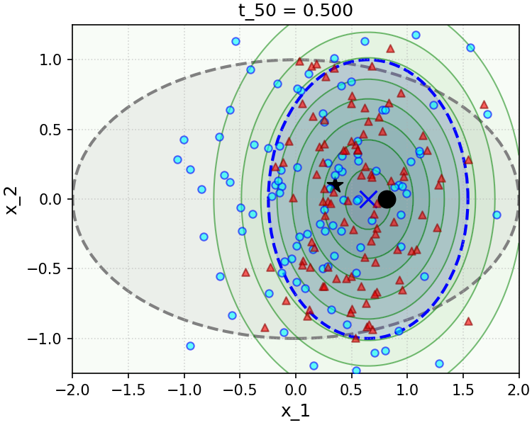


To gain insight into the effect of the convenient approximation (7.3.26), we implement and simulate a simple numerical experiment in the Gaussian setting in Figure 7.11. The sampler we implement is a direct implementation of the simple scheme (3.2.82) we have developed in Chapter 3 and recalled above, using the true conditional posterior denoiser, i.e. Equation (7.3.15) (samples are marked with blue circles), and the convenient approximation to this denoiser made through the measurement matching approximation (7.3.26) (samples are marked with red triangles). The top row of Figure 7.11 shows a setting with large measurement noise \(\sigma ^2\), and the bottom with small measurement noise. The measurement matching approximation works very well in the large-noise setting, with the caveat that in the small-noise setting, it suffers from rapid collapse of the variance of the sampling distribution along directions that are parallel to the rows of the linear measurement operator \(\vA \), which cannot be corrected by later iterations of sampling. Our analysis in Example 7.4 precisely characterizes the level at which the noise becomes too “small” in terms of the data covariance matrix \(\vSigma \).
Generalizing the approximation: Diffusion Posterior Sampling. Example 7.4 suggests a convenient approximation for the measurement matching term, i.e. (7.3.26), which can be made beyond the Gaussian setting of the example. To motivate this approximation in greater generality, notice that by conditional independence of \(\vy \) and \(\vx _t\) given \(\vx \), we can write
Formally, when the posterior \(p_{\vx \mid \vx _t}\) is a delta function centered at its mean \(\bE [\vx \mid \vx _t=\vxi ]\), the approximation (7.3.26) is exact. More generally, when the posterior \(p_{\vx \mid \vx _t}\) is highly concentrated around its mean, the approximation (7.3.26) is accurate. This holds, for example, for sufficiently small \(t\), which we saw explicitly in the Gaussian setting of Example 7.4. Although the numerical simulation in Figure 7.11 suggests that this approximation is not without its caveats in certain regimes, it has proved to be a reliable baseline in practice, after being proposed by Chung et al. as “Diffusion Posterior Sampling” (DPS) [CKM+23]. In addition, there are even principled and generalizable approaches to improve it by incorporating better estimates of the posterior variance (which turn out to be exact in the Gaussian setting of Example 7.4), which we discuss further in the end-of-chapter summary.
Thus, with the DPS approximation, we arrive at the following approximation for the conditional posterior denoisers \(\bE [\vx \mid \vy , \vx _t]\), via 7.3.14:
And, for a neural network or other model \(\bar {\vx }_{\theta }(t, \vxi )\) trained as in Section 3.2 to approximate the denoisers \(\bE [\vx \mid \vx _t = \vxi ]\) for each \(t \in [0, T]\), we arrive at the learned conditional posterior denoisers
Note that the approximation (7.3.28) is valid for arbitrary forward models \(h\) in the observation model (7.3.9), including nonlinear \(h\), and even to arbitrary noise models for which a clean expression for the likelihood \(p_{\vy \mid \vx }\) is known. Indeed, in the case of Gaussian noise, we have
Hence, evaluating the right-hand side of (7.3.29) requires only
Combining this scheme with the basic implementation of unconditional sampling we developed in Section 3.2, we obtain a practical algorithm for conditional sampling of the posterior \(p_{\vx \mid \vy }\) given measurements following (7.3.9). Algorithm 7.1 records this scheme for the case of Gaussian observation noise with known standard deviation \(\sigma \), with minor modifications to extend to a general noising process, as in Equation (3.2.50) and the surrounding discussion in Chapter 3 (our discussion above made the simplifying choices \(\alpha _t = 1\), \(\sigma _t = t\), and \(t_{\ell } = T\ell / L\), as for Equation (3.2.47) in Section 3.2).
Application to medical image reconstruction.
The framework that we have developed above is already powerful enough to be applied to solve various scientific inverse problems, where the measurements \(\vy = h(\vx _o) + \vw \) are the outputs of a known measurement process \(h\) on a specific signal of interest \(\vx _o\), and where there are infinitely many possible signals \(\vx \) that satisfy \(\vy = h(\vx ) + \vw \). This means that to find the true \(\vx _o\) that generated \(\vy \), we need to exploit prior information about the structure of \(\vx _o\). We will consider the probabilistic setting where \(\vx _o \sim p_{\vx }\), and where we have access to a prior on \(p_{\vx }\), say in the form of a diffusion model.
An instructive example of a scientific inverse problem is magnetic resonance imaging (MRI) (Figure 7.12), wherein the data distribution \(p_{\vx }\) is over images corresponding to an underlying object of interest (such as a 2D slice of a human subject’s brain). In MRI applications, the measurement operator \(h\) corresponds to the machine generating and modulating the magnetic field and recording the patient’s response to it (Figure 7.12(c)). It can be modeled as implementing the Fourier transform of the underlying spatial signal (Figure 7.12(a))—see [WM22, Chapter 10] for a detailed mathematical derivation. In addition, for efficiency’s sake, the MRI machine typically only measures a subset of the measured frequencies, in a structured measurement pattern that can be modeled as either a radial or a spiral pattern (Figure 7.12(b)). Writing \(\cF \) to denote the (discrete) Fourier transform operator and \(\cS \) to denote the machine’s (known) subsampling pattern, the measured signal is then
The measurement operator \(\cS \circ \cF \) is linear, implying that it can be represented by a \(m \times n\) matrix after appropriate reshaping, but it is also compressive, which means that \(m \ll n\) and that we need to exploit prior knowledge about \(p_{\vx }\) to reconstruct \(\vx _o\) (or more generally to sample from the posterior \(p_{\vx \mid \vy }\)).
The distribution \(p_{\vx }\) of MRI images is simpler than some image distributions (e.g., natural images), but it is still complex enough to benefit from using a learned model for \(p_{\vx }\) rather than an analytical one (cf. [WM22]). One direct approach is to apply the diffusion posterior sampling approximation we developed in the previous section, which led to Algorithm 7.1, with the specific MRI measurement operator \(\vA = \cS \circ \cF \) and a diffusion model pretrained on MRI data. This precise combination of approaches has not appeared in the literature. Instead, we highlight results from a different but related approach, which enforces measurement consistency on each diffusion step. Following the pioneering work of Song et al. [SSX+22], numerous such measurement consistency algorithms for medical image reconstruction have been developed, including the improved approaches of Song et al. [SKZ+24] and Rout et al. [RRD+23] (which utilize latent diffusion models, as we have developed for representation autoencoders in Chapter 6). Figure 7.13 shows visual comparisons of reconstructed MRI images across three different samples, comparing FISTA-TV (a classical, accelerated version of the ISTA algorithm we studied in Chapter 2), the measurement consistency diffusion modeling approach of Song et al. [SSX+22], and the ground truth. It can be seen that superior reconstruction quality is achieved by the diffusion-based method, as well as superior faithfulness to fine detail in the ground truth image. Table 7.1 shows MRI reconstruction accuracy results (measured in terms of PSNR) for the approach developed by Song et al. [SSX+22]. It compares favorably to supervised baselines (trained on many independent paired samples \((\vy , \vx _o)\), which is an additional requirement) and unsupervised baselines (which correspond to measurement matching approximations that came before diffusion posterior sampling).
| FISTA-TV | Diffusion | Ground Truth |
 |  | |
 |  | |
| Method | \(24\times \) Accel. | \(8\times \) Accel. | \(4\times \) Accel. |
| Cascade DenseNet | \(23.39_{\pm 2.17}\) | \(28.35_{\pm 2.30}\) | \(30.97_{\pm 2.33}\) |
| DuDoRNet | \(18.46_{\pm 3.05}\) | \(\bf 37.88_{\pm 3.03}\) | \(30.53_{\pm 4.13}\) |
| Song et al. [SSK+21] | \(27.83_{\pm 2.73}\) | \(35.04_{\pm 2.11}\) | \(37.55_{\pm 2.08}\) |
| Jalal et al. [JAD+21] | \(28.80_{\pm 3.21}\) | \(36.44_{\pm 2.28}\) | \(38.76_{\pm 2.32}\) |
| Song et al. [SSX+22] | \(\bf 29.42_{\pm 3.03}\) | \(37.63_{\pm 2.70}\) | \(\bf 39.91_{\pm 2.67}\) |
In many practical applications, we do not know either the distribution of the data \(\x \) of interest or the explicit relationship between the data and certain observed attributes \(\y \) of the data. We only have a (large) set of paired samples \((\X , \Y ) = \{ (\x _1, \y _1), \ldots , (\x _N, \y _N) \}\) from which we need to infer the data distribution and a mapping that models their relationship:
The problem of image classification can be viewed as one such example. In a sense, the classification problem is to learn an (extremely lossy) compressive encoder for natural images. Say, given a random sample of an image \(\x \), we would like to predict its class label \(\y \) that best correlates the content in \(\x \). We know the distribution of natural images of objects is low-dimensional compared to the dimension of the pixel space. From the previous chapters, we have learned that given sufficient samples, in principle, we can learn a structured low-dimensional representation \(\z \) for \(\x \) through a learned compressive encoding:
The representation \(\z \) can also be viewed as a learned (lossy but structured) code for \(\x \). It is rather reasonable to assume that if the class assignment \(\y \) truly depends on the low-dimensional structures of \(\x \) and the learned code \(\z \) truly reflects such structures, \(\y \) and \(\z \) can be made highly correlated and hence their joint distribution \(p(\z , \y )\) should be extremely low-dimensional. Therefore, we may combine the two desired codes \(\y \) and \(\z \) together and try to learn a combined encoder:
where the joint distribution of \((\z , \y )\) is highly low-dimensional.
From our study in previous chapters, the mapping \(f\) is usually learned as a sequence of compression or denoising operators in the same space. Hence to leverage such a family of operations, we may introduce an auxiliary vector \(\vw \) that can be viewed as an initial random guess of the class label \(\y \). In this way, we can learn a compression or denoising mapping:
within a common space. In fact, the common practice of introducing an auxiliary “class token” in the training of a transformer for classification tasks, such as in ViT, can be viewed as learning such a representation by compressing (the coding rate of) given (noisy) samples of \((\x , \vw )\). If the distribution of the data \(\x \) is already a mixture of (low-dimensional) Gaussians, the work [WTL+08] has shown that classification can be done effectively by directly minimizing the (lossy) coding length associated with the given samples.
While a learned classifier allows us to classify a given image \(\x \) to its corresponding class, we often would like to generate an image of a given class, by sampling the learned distribution of natural images. To some extent, this can be viewed as the “inverse” problem to image classification. Let \(p_{\x }\) denote the distribution of natural images, say modeled by a diffusion-denoising process. Given a class label random variable \(y \in [K]\) with realization \(\nu \), say an “Apple”, we would like to sample the conditional distribution \(p_{\x \mid y}(\,\cdot \, \mid \nu )\) to generate an image of an apple:
We call this class-conditioned image generation.
In Section 7.3.2, we have seen how to use the denoising-diffusion paradigm for conditional sampling from the posterior \(p_{\vx \mid \vy }\) given model-based measurements \(\vy = h(\vx ) + \vw \) (Equation (7.3.9)), culminating in the DPS algorithm (Algorithm 7.1). This is a powerful framework, but it does not apply to the class (or text) conditioned image generation problem here, where an explicit generative model \(h\) for the observations/attributes \(y\) is not available due to the intractability of analytical modeling. In this section, we will present techniques for extending conditional sampling to this setting.
Thus, we now assume only that we have access to samples from the joint distribution of \((\vx , y)\):
As in the previous section, we define \(\vx _t = \alpha _t \vx + \sigma _t \vg \) with \(\vg \sim \cN (\Zero , \vI )\) independent of \((\vx , \vy )\), as in Equation (3.2.50) in Chapter 3, and we will repeatedly use the notation \(\vxi \) to denote realizations of \(\vx \) and \(\vx _t\).
This section focuses on the conceptual and algorithmic underpinnings for conditional sampling in modern generative models. For a treatment focused on implementation issues in various applications, see Chapter 8, Section 8.7 and subsequent sections.
Recall from Section 7.3.2 that the following decomposition of the optimal conditional posterior denoiser holds, by virtue of Bayes’ rule and conditional independence of \(\vy \) and \(\vx _t\) given \(\vx \) (recall Figure 7.10):
In other words, the representation (7.4.7) for the optimal conditional denoiser holds regardless of whether the explicit observation model \(\vy = h(\vx ) + \vw \) is valid. This means that if we can learn such a denoiser (7.4.7) in the paired data setting, we can follow the denoising-diffusion methodology we have developed in Chapter 3 to perform class-conditional sampling.
A natural idea is then to directly implement the likelihood correction term in (7.4.7) using a deep network \(f_{\theta _{\mathrm {c}}}\) with parameters \(\theta _{\mathrm {c}}\), as in Equation (7.4.4):
This expression combines the final representations \(\vz (t, \vx _t)\) (which also depend on \(\theta _{\mathrm {c}}\)) of the noisy inputs \(\vx _t\) with a classification head \(\vW _{\mathrm {head}} \in \bR ^{K \times d}\), which maps the representations to a probability distribution over the \(K\) possible classes. As is common in practice, it also takes the time \(t\) in the noising process as input. Thus, with appropriate training, it provides an approximation to the log-likelihood \(\log p_{y \mid \vx _t}\), and differentiating \(\log f_{\theta _{\mathrm {c}}}\) with respect to its input \(\vx _t\) allows an approximation to the second term in Equation (7.4.7):
where, as usual, we approximate the first term in Equation (7.4.7) via a learned unconditional denoiser for \(\vx _t\) with parameters \(\theta _{\mathrm {d}}\), and where we write \(\ve _k\) for \(k \in [K]\) to denote the \(k\)-th canonical basis vector for \(\R ^K\) (i.e., the vector with a one in the \(k\)-th position, and zeros elsewhere). The reader should note that the conditional denoiser \(\bar {\vx }_{\theta }\) requires two separate training runs, with separate losses: one for the classifier parameters \(\theta _{\mathrm {c}}\), on a classification loss,7 and one for the denoiser parameters \(\theta _{\mathrm {d}}\), on a denoising loss. Such an approach to conditional sampling was already recognized and exploited to perform conditional sampling in pioneering early works on diffusion models, notably those by Sohl-Dickstein et al. [SWM+15] and by Song et al. [SSK+21].
However, this straightforward methodology has two key drawbacks (which is why we label it as “naive”). The first is that, empirically, such a trained deep network classifier frequently does not provide a strong enough guidance signal (in Equation (7.4.7)) to ensure that generated samples reflect the conditioning information \(y\). This was first emphasized by Dhariwal and Nichol [DN21b], who noted that in the setting of class-conditional ImageNet generation, the learned deep network classifier’s probability outputs for the class \(y\) being conditioned on were frequently around \(0.5\)—large enough to be the dominant class, but not large enough to provide a strong guidance signal—and that upon inspection, generations were not consistent with the conditioning class \(y\). Dhariwal and Nichol [DN21b] proposed to address this heuristically by incorporating an “inverse temperature” hyperparameter \(\gamma > 0\) into the definition of the naive conditional denoiser (7.4.9), referring to the resulting conditional denoiser as having incorporated “classifier guidance” (CG):
with the case \(\gamma = 1\) coinciding with (7.4.9).
Dhariwal and Nichol [DN21b] found that a setting \(\gamma > 1\) performed best empirically. One possible interpretation for this is as follows: note that, in the context of the true likelihood term Equation (7.4.7), scaling by \(\gamma \) gives equivalently
which suggests the natural interpretation of the parameter \(\gamma \) performing (inverse) temperature scaling on the likelihood \(p_{\vy \mid \vx _t}\), which is precise if we consider the renormalized distribution \( { p_{\vy \mid \vx _t}(\vnu \mid \vxi )^\gamma } / { \int p_{\vy \mid \vx _t}(\vnu '\mid \vxi )^\gamma \odif \vnu ' } \). However, note that this is not a rigorous interpretation in the context of Equation (7.4.7), because the gradients are taken with respect to \(\vxi \), and the normalization constant in the temperature-scaled distribution is in general a function of \(\vxi \). Instead, the parameter \(\gamma \) should simply be understood as amplifying large values of the deep network classifier’s output probabilities \(f_{\theta _{\mathrm {c}}}(t, \vx _t)\) relative to smaller ones, which effectively amplifies the guidance signal provided in cases where the deep network \(f\) assigns it the largest probability among the \(K\) classes.
Nevertheless, classifier guidance does not address the second key drawback of the naive methodology: it is both cumbersome and wasteful to have to train an auxiliary classifier \(f_{\theta _{\mathrm {c}}}\) in addition to the unconditional denoiser \(\bar {\vx }_{\theta _{\mathrm {d}}}\), given that it is not possible to directly adapt a pretrained classifier due to the need for it to work well on noisy inputs \(\vx _t\) and incorporate other empirically-motivated architecture modifications. In particular, Dhariwal and Nichol [DN21b] found that it was necessary to explicitly design the architecture of the deep network implementing the classifier to match that of the denoiser.
Moreover, from a purely practical perspective—trying to obtain the best possible performance from the resulting sampler—the best-performing configuration of classifier guidance-based sampling departs even further from the idealized and conceptually sound framework we have presented above. To obtain the best performance, Dhariwal and Nichol [DN21b] found it necessary to provide the class label \(y\) as an additional input to the denoiser \(\bar {\vx }_{\theta _{\mathrm {d}}}\). As a result, the idealized classifier-guided denoiser (7.4.10), derived by Dhariwal and Nichol [DN21b] as we have done above from the conditional posterior denoiser decomposition (7.4.7), is not exactly reflective of the best-performing denoiser in practice—such a denoiser actually combines a conditional denoiser for \(\vx _t\) given \(y\) with an additional guidance signal from an auxiliary classifier!
This state of affairs, empirically motivated as it is, led Ho and Salimans [HS22a] in subsequent work to propose a more empirically pragmatic methodology, known as classifier-free guidance (CFG). Instead of representing the conditional denoiser (7.4.7) as a weighted sum of an unconditional denoiser for \(\vx _t\) with a log-likelihood correction term (with possibly modified weights, as in classifier guidance), they accept the apparent necessity of training a conditional denoiser for \(\vx _t\) given \(y\), as demonstrated by the experimental results of Dhariwal and Nichol [DN21b], and replace the log-likelihood gradient term with a correctly-weighted sum of this conditional denoiser with an unconditional denoiser for \(\vx \) given \(\vx _t\).8
Deriving Classifier-Free Guidance. To see how this structure arises, we begin with an ‘idealized’ version of the classifier guidance denoiser \(\bar {\vx }_{\theta }^{\mathrm {CG}}\) defined in (7.4.10), for which the denoiser \(\bar {\vx }_{\theta _{\mathrm {d}}}\) and the classifier \(f_{\theta _{\mathrm {c}}}\) perfectly approximate their targets, via (7.4.7):
We then use Bayes’ rule, in the form
together with Tweedie’s formula (Theorem 3.2, modified as in Equation (3.2.51)) to convert between score functions and denoisers, to obtain
where in the last line, we apply Equation (7.3.11). Now, 7.4.14 suggests a natural approximation strategy: we combine a learned unconditional denoiser for \(\vx \) given \(\vx _t\), as previously, with a learned conditional denoiser for \(\vx \) given \(\vx _t\) and \(y\).
However, following Ho and Salimans [HS22a] and the common practice of training deep network denoisers, it is standard to use the same deep network to represent both the conditional and unconditional denoisers by introducing an additional label, which we will denote by \(\varnothing \), to denote the “unconditional” case. This leads to the form of the CFG denoiser:
To train a denoiser \(\bar {\vx }_{\theta }(t, \vx _t, y^+)\) for use with classifier-free guidance sampling, where \(y^+ \in \set {1, \dots , K, \varnothing }\), we proceed almost identically to the unconditional training procedure in Algorithm 3.2, but with two modifications:
In this way, we train a conditional denoiser suitable for use in classifier-free guidance sampling. We summarize the overall sampling process for class-conditioned sampling with classifier-free guidance in Algorithm 7.2.
Ho and Salimans [HS22a] reports strong empirical performance for class-conditional image generation with classifier-free guidance, and it has become a mainstay of the largest-scale practical diffusion models, such as Stable Diffusion [RBL+22] and its derivatives.
What Denoisers Does Classifier-Free Guidance Promote Learning? As we have seen, the derivation of classifier-free guidance is rather opaque and empirically motivated, giving little insight into the mechanisms behind its strong performance. A number of theoretical works have attempted to address this [BN24b; LWQ25; WCL+24]. They provide explanations for some parts of the overall CFG methodology—itself encompassing denoiser parameterization and training, as well as configuration of the guidance strength and performance at sampling time. Below, following our running theme in the book, we will give an interpretation in the simplifying setting of a Gaussian mixture model data distribution and denoiser. First, we consider the effect of CFG: what does a large weight \(\gamma \gg 1\) promote?
Example 7.5. Let us recall the low-rank mixture of Gaussians data generating process we studied in Example 3.3 (and specifically, the form in Equation (3.2.40)). Given \(K \in \bN \) classes, we assume that
Applying the analysis in Example 3.3 (and the subsequent analysis of the low-rank case, culminating in Equation (3.2.45)), we obtain for the class-conditional optimal denoisers
This denoiser has a simple, interpretable form:
The CFG scheme averages these two denoisers. The effect of this averaging can be gleaned from the refactoring
This implies: if the CFG denoiser’s input is highly correlated with one of the class subspaces, the denoiser is approximately equal to the corresponding class-conditional denoiser! Hence, we expect the CFG denoising sampler to converge.
Meanwhile, in the second term of Equation (7.4.20), any classes \(k \neq y\) that are well-correlated with \(\vx _t\) receive a large negative weight from the \(1 - \gamma \) coefficient. This simultaneously has the effect of making the denoised signal vastly more correlated with the conditioning class \(y\), and making it negatively correlated with the previous iterate (i.e., the iterate before denoising).
In other words, CFG steers the iterative denoising process towards the conditioning class and away from the previous iterate, a different dynamics from purely conditional sampling (i.e., the case \(\gamma = 1\)).
Example 7.5 shows that in the mixture of Gaussians setting, the CFG denoiser provides a strong bias towards the conditioning class, while preserving local correctness (hence convergence of sampling) when the noise level \(t\) is small. This is suggestive of why a large weight \(\gamma \gg 1\) has been found essential in practice.
Next, the following example will demonstrate an insight into the parameterization of the denoiser in the presence of low-dimensional structure, again in the Gaussian mixture model.
Example 7.6. Consider again the mixture of Gaussians model studied in Example 7.5:
Now we consider the problem of parameterizing a learnable denoiser \(\vx _{\theta }^{\mathrm {CFG}}\) to represent the optimal denoiser (7.4.26). For tractability, we add an additional assumption associated to the subspaces \(\vU _k\) being ‘distinguishable’ from one another, which is natural in practice: specifically, we assume that for any pair of indices \(k, k' \in [K]\) with \(k \neq k'\), we can find a set of \(K\) nonzero directions \(\vv _{k} \in \bR ^D\) such that
These vectors \(\vv _k\) can then be thought of as embeddings of the class label \(y \in [K]\), and we can use them to define a more general operator that can represent both the unconditional and class-conditional denoisers. More precisely, consider the mapping
We aim to simplify the preceding expression further. To this end, recall that when using this denoiser for sampling, we have \(\vx _t = \vx + t \vg \), with \(y\) denoting the label of \(\vx \). In other words, conditioned on \(y\), we have that \(\vx _t = \vU _y \vz + t \vg \), where \(\vz \) is an independent \(P\)-dimensional Gaussian noise vector with zero mean and identity covariance. We have
Because \(\vz \) and \(\vg \) are independent Gaussian random variables with identity covariance matrices, it follows from rotational invariance of the Gaussian distribution (see [Ver18]) that
where \(z\) and \(g\) are independent scalar \(\cN (0, 1)\) random variables, and \(\equid \) denotes equality in distribution (the random variables have the same distribution). The second line above follows from the definition of \(\vv _y\). Now, by independence, the random variable \(z + tg \sim \cN (0, (1 + t^2))\). Then using the well-known result that \(\bE [\abs {g}] = \sqrt {2/\pi }\) if \(g \sim \cN (0, 1)\), we conclude
Thus, the family of operators (7.4.28) provides a unified way to parameterize the constituent operators in the optimal denoiser for \(\vx \) within a single ‘network’. More precisely, it is enough to add the output of an instantiation of (7.4.28) with input \((\vx _t, \vx _t)\) to an instantiation with input \((\vx _t, \vv _{t, y})\). The resulting operator is a function of \((t, \vx _t, y)\), and computationally, the subspaces \((\vU _k)_{k=1}^K\) and embeddings \(y \mapsto \vv _{t, y}\) become its learnable parameters. \(\blacksquare \)
Example 7.6 shows that in the special case of a low-rank mixture of Gaussians data distribution for \(\vx \) with incoherent components, operators of the form
provide a sufficiently rich class of operators to parameterize the ideal denoiser for noisy observations \(\vx _t\) of \(\vx \) when using classifier-free guidance. For such operators, the auxiliary input \(\vv \) can be taken as either \(\vx _t\) or a suitable embedding of the class label \(y \mapsto \vv _y\) in order to realize such a denoiser—as the example shows, the ideal denoiser is a weighted sum of such operators, with weights derived from the guidance strength \(\gamma >1\).
Based on the framework in Chapter 5, which develops deep network architectures suitable for transforming more general data distributions to structured representations using the low-rank mixture of Gaussians model as a primitive, it is natural to imagine that operators of the type (7.4.32) may be leveraged in denoisers for general data distributions \(\vx \) with low-dimensional geometrically-structured components that are sufficiently distinguishable (say, incoherent) from one another. The next section demonstrates that this is indeed the case.
In Section 7.4.1 we have seen, conceptually, how to set up denoisers for use with classifier-free guidance, the dominant practical methodology for performing conditional sampling via the diffusion-denoising paradigm. In short, such denoisers take as input the noisy data \(\vx _t\) as well as either the conditioning signal \(\vy \) or a “null input” \(\varnothing \), which determines whether the denoiser should perform unconditional denoising or conditional denoising (conditioned on \(\vy \)).
Given this design, the most important practical question is how to realize this family of operators as a neural network? An empirically-successful neural network layer design known as “cross attention”, which we will present in due course, provides a practical answer to this question. However, even before this, there are several more fundamental issues to sort out:
We will cover these three issues in detail below, providing guidance on how to explore the design space and, where possible, generally-useful prescriptions.
Although we do not know the precise relationship between \(\vx \) and \(\vy \) in the general paired data setting, in all practical settings of interest, they have significant correlations. For example, when the conditioning signal \(\vy \) is a “caption” describing the image \(\vx \) in natural language, it is easy to imagine a human artist being able to produce an accurate sketch of \(\vx \) based solely on a high-quality caption. In our probabilistic setting, one natural way to quantify these “correlations” is in terms of the mutual information, which we saw previously in Chapter 4 (Equation (4.1.9)):
The mutual information (7.4.33) is a purely information-theoretic quantity that does not depend on modality-specific aspects of \(\vx \) and \(\vy \). Hence it offers a natural criterion for learning a useful representation of either input \(\vx \), \(\vy \): one simply seeks to learn, say for \(\vx \), a representation \(\vz = f(\vx )\) that preserves the mutual information, so that \(I(\vz ; \vy ) \approx I(\vx ; \vy )\). That is:
Actually, we can be even more prescriptive here. For an encoder \(f\) which is deterministic (matching all the cases we have studied throughout Chapters 4 and 6), a fundamental result in information theory known as the data processing inequality tells us that processing \(\vx \) with \(f\) to produce \(\vz = f(\vx )\) changes the mutual information in a predictable way: it can only reduce it.
Theorem 7.1 (Data Processing Inequality). Consider random variables \(\vy , \vx , \vz \) defined such that \(\vz \) is independent of \(\vy \), conditioned on \(\vx \).11 Then the data processing inequality holds:
Proof. Consider the mutual information \(I(\vy ; \vx , \vz )\) between \(\vy \) and \((\vx , \vz )\). Because \(\vz \) is independent of \(\vy \) conditioned on \(\vx \), we have
For a deterministic encoder \(f\), \(\vz = f(\vx )\) is always independent of \(\vy \) when conditioned on \(\vx \). The data processing inequality therefore suggests the following computational procedure to find the encoder \(f\): seek to maximize the mutual information between the representation and the conditioning signal. Equation (7.4.31) then leads to the objective
This is known as the Infomax principle [Lin88], and it dates to the earliest years of representation learning.
Computational considerations in applying the Infomax principle. There are two key conceptual issues to keep in mind when thinking about how to apply the (abstract) Infomax principle (7.4.36) for learning a representation. The first is that in general it is computationally hard to estimate the mutual information, which constitutes the objective in (7.4.36). As we discussed in the context of rate distortion and lossy coding when we introduced the mutual information in Chapter 4, the mutual information can be relaxed to remain well-defined even when \(\vx \) and \(\vy \) are low-dimensional and have differential entropy approaching \(-\infty \) (e.g., by connection to the Gaussian rate reduction function that we have studied in Chapters 4 to 6). Moreover, empirically such relaxations have non-worst-case statistical properties in practice, as we saw in the experiments of Chapter 4; and the accuracy of these approximations can be improved by incremental processing, as we saw in Chapter 5. This makes a criterion like Equation (7.4.33) an excellent foundation for learning representations of paired data \((\vx , \vy )\).
The second issue to keep in mind is that for the objective (7.4.36) to represent a sensible criterion for learning \(f\), it is necessary that \(f\) itself is parameterized in a specific way, and/or that some additional structural enforcement is done on the representations \(f(\vx )\). Indeed, if \(f\) is completely unconstrained, there are simple trivial solutions to (7.4.36) that do not correspond to useful representations: for example, just take \(f(\vx ) = \vx \) to be the identity! We discussed principled techniques for structuring the representation space in Chapter 6 when we discussed autoencoding and closed loop transcription; many of these techniques can be brought to bear in our present joint embedding setting, and we will detail this further later in the section, when we move to practical implementation.
Joint embedding with the Infomax principle. Now, the question of joint representation of \((\vx , \vy )\) remains. Applying the data processing inequality once more, we obtain for another encoder \(g\) that produces a representation of \(\vy \) that
The joint objective
is then a well-founded consequence of the Infomax principle.
To design the encoders \(f\) and \(g\), recall the intuition that we obtained through our work in Example 7.6. There, we saw that in the case of a mixture-of-Gaussians model for \(\vx \), with the conditioning signal \(y\) identifying which specific mixture component generates the observation, a flexible denoiser architecture could be constructed via a suitable embedding of the class label \(y\) into the same space as the data \(\vx \). More precisely, such an embedding \(\vu _y \in \R ^D\) allows, when correlated with the embeddings \(\vU _{\vx }\) of \(\vx \in \R ^{D}\) (generally a matrix) via \(\vu _y^\top \vU _{\vx }\), to ‘pick out’ only the embeddings relevant to the correct mixture component of the distribution. How exactly to design these layers for use in neural networks being trained on more complex nonlinear high-dimensional data is a challenging question that we will dig into in more detail below. But a necessary condition is clear: the embeddings \(f\) and \(g\) should map their inputs to a common embedding space, say \(\R ^d\), to facilitate downstream comparison when performing conditional sampling. This leads to the objective
The next step is to instantiate a suitable computationally-convenient relaxation of the mutual information in (7.4.38) for use with large-scale datasets.
A concrete and highly influential realization of learning joint embeddings for paired data is the method of Contrastive Language-Image Pre-training (CLIP) [RKH+21b]. Take the simple case of image-text pairs \([(\x _i, \y _i)]_{i=1}^N\) sampled from a dataset \(\mathcal {D}\), where \(\x _i\) is an image and \(\y _i\) is a text caption. CLIP trains two encoders—an image encoder \(f_{\theta }(\x )\) and a text encoder \(g_{\plainphi }(\y )\)—to map paired samples into a shared \(d\)-dimensional unit sphere (i.e. \(\|f_{\theta }(\x _i)\|_2 = 1\) and \(\|g_{\plainphi }(\y _i)\|_2 = 1\)). To achieve this, we can adopt a simple symmetric cross-entropy loss that pushes the cosine similarity of matched pairs \((f_{\theta }(\x _i),g_{\plainphi }(\y _i))\) closer together while repelling unmatched pairs:
From the perspective of mutual information maximization, CLIP is a tractable surrogate for the lower bound on the mutual information between the image and text representations:12
Thus, CLIP provides a practical recipe for learning joint embeddings for paired data that increases the mutual information between the paired samples. Empirically, CLIP has been shown to be effective at learning joint embeddings for image-text pairs, and has been used in a variety of applications, including image captioning, image-text retrieval, image generation and beyond. We will see more specific examples in Chapter 8 (with key implementation details described in detail in Section 8.3).
Finally, we will describe an end-to-end system that integrates joint image-text encoders, learned with the CLIP loss as described above, with conditioning operators that are evocative of the mixture-of-Gaussians operator (7.4.32) we saw in Example 7.6. These techniques formed the basis for the original open-source Stable Diffusion implementation [RBL+22], where the embedding and subsequent conditioning is performed not on a class label, but a text prompt, which describes the desired image content (Figure 7.14). This section will give a high-level overview of StableDiffusion-style image generation. For full implementation details sufficient to re-implement such a system from scratch, we refer to Chapter 8: specifically, Section 8.11 describes the process of encoding strings of text to a sequence of integer IDs; Section 8.3 describes the training of the necessary image-text encoders; and Sections 8.6 and 8.7 describe the training of the (latent) diffusion model.
Stable Diffusion follows the conditional generation methodology we outline in Section 7.4.1, with two key modifications: (i) The conditioning signal is a tokenized text prompt \(\vY \in \bR ^{D_{\mathrm {text}} \times N}\), rather than a class label; (ii) Image denoising is performed in “latent” space rather than on raw pixels, using a specialized, pretrained variational autoencoder pair \(f : \bR ^{D_{\mathrm {img}}} \to \bR ^{d_{\mathrm {img}}}\), \(g : \bR ^{d_{\mathrm {img}}} \to \bR ^{D_{\mathrm {img}}}\) (see Sections 6.1.4 and 8.6), where \(f\) is the encoder and \(g\) is the decoder. For issue (i), in the context of the iterative conditional denoising framework we have developed in Section 7.4.1, this concerns the parameterization of the denoisers \(\bar {\vz }_{\theta }(t, \vz _t, \vY ^+)\).13 Rombach et al. [RBL+22] implement text conditioning in the denoiser using a layer known as cross attention, inspired by the original encoder-decoder transformer architecture of Vaswani et al. [VSP+17b]. Cross attention is implemented as follows. We let \(\tau : \bR ^{D_{\mathrm {text}} \times N} \to \bR ^{d_{\mathrm {model}} \times N_{\mathrm {text}}}\) denote an encoding network for the text embeddings (often a causal transformer—see Section 8.11), and let \(\psi : \bR ^{d_{\mathrm {img}}} \to \bR ^{d_{\mathrm {model}} \times N_{\mathrm {img}}}\) denote the mapping corresponding to one of the intermediate representations in the denoiser.14 Here, \(N_{\mathrm {text}}\) is the maximum tokenized text prompt length, and \(N_{\mathrm {img}}\) roughly corresponds to the number of image channels (layer-dependent) in the representation, which is fixed if the input image resolution is fixed. Cross attention (with \(K\) heads, and no bias) is defined as
where \(\mathrm {SA}\) denotes the scaled dot-product attention operation in the transformer (which we recall in detail in Chapter 8: see Equation (8.2.13) and 8.2.18), and \(\vU _{*}^{k} \in \bR ^{d_{\mathrm {model}}\times d_{\mathrm {attn}} }\) for \(* \in \set {\mathrm {qry}, \mathrm {key}, \mathrm {val}}\) (as well as the output projection \(\vU _{\mathrm {out}}\)) are the learnable parameters of the layer.
Notice that, by the definition of the self-attention operation, cross attention outputs linear combinations of the value-projected text embeddings weighted by correlations between the image features and the text embeddings. In the denoiser architecture used by Rombach et al. [RBL+22], self-attention residual blocks in the denoiser architecture, applied to the image representation at the current layer and defined analogously to those in Equation (8.2.12) for the vision transformer, are followed by cross attention residual blocks of the form (7.4.41). Such a structure requires the text encoder \(\tau \) to, in a certain sense, share some structure in its output with the image feature embedding \(\psi \): this can be achieved via joint embedding, learned by a procedure such as CLIP as described above. Conceptually, this joint text-image embedding space and the cross attention layer itself bear a strong resemblance to the conditional mixture of Gaussians denoiser that we derived in the previous section (recall (7.4.28)), in the special case of a single token sequence. Deeper connections can be drawn in the multi-token setting following the rate reduction framework for deriving deep network architectures discussed in Chapter 5, and manifested in the derivation of the CRATE transformer-like architecture.
This same basic design has been further scaled to even larger model and dataset sizes, in particular in modern instantiations of Stable Diffusion [EKB+24], as well as in competing models such as FLUX.1 [LBB+25], Imagen [SCS+22], and DALL-E [RDN+22]. The conditioning mechanism of cross attention has also become ubiquitous in other applications, as in EgoAllo (Section 8.10) for conditioned pose generation and in Michelangelo (Section 8.8) for conditional 3D shape generation based on images or texts.
In this last section, we consider the more extreme, but actually ubiquitous, case for distribution learning in which we only have a set of observed samples \(\Y = \{\y _1,\ldots , \y _N\}\) of the data \(\x \), but no samples of \(\x \) directly! In general, the observation \(\y \in \mathbb {R}^d\) is of lower dimension than \(\x \in \mathbb {R}^D\). To make the problem well-defined, we do assume that the observation model between \(\y \) and \(\x \) is known to belong to a certain family of analytical models, denoted as \(\y = h(\x , \theta ) +\vw \), with \(\theta \) either known or not known.
Let us first try to understand the problem conceptually with the simple case when the measurement function \(h\) is known and the observed \(\y = h(\x ) + \vw \) is informative about \(\x \). That is, we assume that \(h\) is surjective from the space of \(\x \) to that of \(\y \) and the support of the distribution \(\y _0 = h(\x _0)\) is low-dimensional. This typically requires that the extrinsic dimension \(d\) of \(\y \) is higher than the intrinsic dimension of the support of the distribution of \(\x \). Without loss of generality, we may assume that there exist functions:
Notice that here we may assume that we know \(G(\y )\) but not \(F(\x )\). Let \(\mathcal {S}_{\y } \doteq \{\y \mid G(\y ) = \boldsymbol {0}\}\) be the support of \(p(\y )\). In general, \(h^{-1}(\mathcal {S}_{\y }) = \{\x \mid G(h(\x )) = \boldsymbol {0}\}\) is a superset of \(\mathcal {S}_{\x } \doteq \{\x \mid F(\x ) = \boldsymbol {0}\}\). That is, we have \(h(\mathcal {S}_{\x }) \subseteq \mathcal {S}_{\y }\).
First, for simplicity, let us consider that the measurement is a linear function of the data \(\x \) of interest:
Here the matrix \(\vA \in \mathbb {R}^{m\times n}\) is of full row rank and \(m\) is typically smaller than \(n\). We assume \(\vA \) is known for now. We are interested in how to learn the distribution of \(\x \) from such measurements. Since we no longer have direct samples of \(\x \), we wonder whether we can still develop a denoiser for \(\x \) with observations \(\y \). Let us consider the following diffusion process:
where \(\vg \sim \mathcal {N}(\boldsymbol {0}, \vI )\).
Without loss of generality, we assume \(\vA \) is of full row rank, i.e., under-determined. Let us define the corresponding process \(\x _t\) as one that satisfies:
From the denoising process of \(\y _t\), we have
for a small \(s >0\). So \(\x _{t-s}\) and \(\x _t\) need to satisfy:
Among all \(\x _{t-s}\) that satisfy the above constraint, we arbitrarily choose the one that minimizes the distance \(\|\x _{t-s} - \x _t\|_2^2\). Therefore, we obtain a “denoising” process for \(\x _t\):
Notice that this process does not sample from the distribution of \(\vx _t\). In particular, there are components of \(\vx \) in the null space/kernel of \(\vA \) that can never be recovered from observations. Thus more information is needed to recover the full distribution of \(\vx \), strictly speaking. But this recovers the component of \(\vx \) that is orthogonal to the null space of \(\vA \).
In practice, the measurement model is often nonlinear or only partially known. A typical problem of this kind is actually behind how we can learn a working model of the external world from the images perceived, say through our eyes, telescopes or microscopes. In particular, humans and animals are able to build a model of the 3D world (or 4D for a dynamical world) through a sequence of its 2D projections—a sequence of 2D images (or stereo image pairs). The mathematical or geometric model of the projection is generally known:
where \(h(\cdot )\) represents a (perspective) projection of the 3D (or 4D) scene from a certain camera view at time \(t_i\) to a 2D image (or a stereo pair) and \(\vw \) is some possibly additive small measurement noise. Figure 7.15 illustrates this relationship concretely, while Figure 7.16 illustrates the model problem in the abstract. A full exposition of geometry related to multiple 2D views of a 3D scene is beyond the scope of this book. Interested readers may refer to the book [MKS+04]. For now, all we need to proceed is that such projections are well understood and multiple images of a scene contain sufficient information about the scene.
In general, we would like to learn the distribution \(p(\x )\) of the 3D (or 4D) world scene \(\x \)15 from the perceived 2D images of the world so far. The primary function of such a (visual) world model is to allow us to recognize places where we had been before or predict what the current scene would look like in a future time at a new viewpoint.
Let us first examine the special but important case of stereo vision. In this case, we have two calibrated views of the 3D scene \(\x \):
where parameters \(\theta ^0\) and \(\theta ^1\) for the view poses can be assumed to be known. \(\y ^0\) and \(\y ^1\) are two 2D-projections of the 3D scene \(\x \). We may also assume that they have the same marginal distribution \(p(\y )\) and we have learned a diffusion and denoising model for it. That is, we know the denoiser:
Or, furthermore, we may assume that we have a sufficient number of samples of stereo pairs \((\y ^0, \y ^1)\) and have also learned the joint distribution of the pairs. By a little abuse of notation, we also use \(\y = h(\x )\) to indicate the pair \(\y = (\y ^0, \y ^1)\) and \(p(\y )\) as the learned probability distribution of the pair (say via a denoiser as above).
The main question now is: How to learn (a representation for) the distribution of the 3D scene \(\x \) from its two projections with known relationships? People might question the rationale for doing this: why is this necessary if the function \(h(\cdot )\) is largely invertible? That is, the observation \(\y \) can largely determine the unknown \(\x \), which is kind of the case for stereo—in general, two (calibrated) images contain sufficient information about the scene depth, from the given vantage point. However, 2D images are far from the most compact representation of the 3D scene as the same scene can produce infinitely many (highly correlated) 2D images or image pairs. In fact, a good representation of a 3D scene should be invariant to the viewpoint. Hence, a correct representation of the distribution of 3D scenes should be much more compact and structured than the distribution of 2D images, stereo pairs, or image-depth pairs.
Consider the (inverse) denoising process for the diffusion: \(\y _t = \y + t\vg \) in (7.5.11), where \(\vg \) is standard Gaussian. From the denoising process of (7.5.11), we have
We try to find a corresponding “denoising” process of \(\x _t\) such that \(\x \) is related to \(\y \) as:
Then we have:
for a small \(s >0\). Suppose \(\x _{t-s} = \x _t + s \vv \) for some vector \(\vv \) and small increment \(s\). We have
Geometrically the vector \(\vv \) in the domain of \(\x \) can be viewed as the pullback of the vector field \(t \nabla \log p_t(\y )\) under the map \(\y = h(\x )\). In general, as before, we may (arbitrarily) choose \(\vv \) to be the minimum 2-norm vector that satisfies the pullback relationship. Hence, we can express \(\hat {\x }_{t-s}\) approximately as:
Remark 7.2 (Parallel Sensing and Distributed Denoising.). There is something very interesting about the above equation (7.5.17). It seems to suggest we could try to learn the distribution of \(\x \) through a process that is coupled with (many of) its (partial) observations:
Visual World Model from Uncalibrated Image Sequences. In the above derivation, we have assumed that the measurement model \(h(\cdot )\) is fully known. In the case of stereo vision, this is rather reasonable as the relative pose (and calibration) of the two camera views (or two eyes16) is usually known in advance. Hence, through the stereo image pairs, in principle we should be able to learn the distribution of 3D scenes, at least the ego-centric distribution of 3D scenes. However, the low-dimensional structures of the so-called learned distribution contain variation caused by changing the viewpoints. That is, the appearance of the stereo images varies when we change our viewpoints with respect to the same 3D scene. For many practical vision tasks (such as localization and navigation), it is important that we can decouple this variation of viewpoints from an invariant representation of (the distribution of) 3D scenes.
Remark 7.3. Note that the above goal aligns well with Klein’s Erlangen Program for modern geometry, which is to study invariants of a manifold under a group of transformations. Here, we may view the manifold of interest as the distribution of ego-centric representations of 3D scenes. We have learned that it admits a group of three-dimensional rigid-body motion acting on it. It is remarkable that our brain has learned to effectively decouple such transformations from the observed 3D world.
Notice that we have studied learning representations that are invariant to translation and rotation in a limited setting in Chapter 5. We know that the associated compression operators take the necessary form of (multi-channel) convolutions, hence leading to the (deep) convolutional neural networks. Nevertheless, operators that are associated with compression or denoising that are invariant to more general transformation groups remain elusive to characterize [CW16b]. For the 3D Vision problem in its most general setting, we know the change of our viewpoints can be well modeled as a rigid-body motion. However, the exact relative motion of our eyes between different viewpoints is usually not known. More generally, there could also be objects (e.g., cars, humans, hands) moving in the scene and we normally do not know their motion either. How can we generalize the problem of learning the distribution of 3D scenes with calibrated stereo pairs to such more general settings? More precisely, we want to learn a compact representation \(\x \) of the 3D scenes that is invariant to the camera/eye motions. Once such a representation is learned, we could sample and generate a 3D scene and render images or stereo pairs from arbitrary poses.
To this end, note that we can model a sequence of stereo pairs as:
where \(h(\cdot )\) represents the projection map from 3D to 2D. \(\theta ^k\) denotes the rigid-body motion parameters of the \(k\)th view, with respect to some canonical frame in the world. \(\x ^k\) represents the 3D scene at time \(k\). If the scene is static, \(\x ^k\) should all be the same \(\x ^k = \x \). To simplify the notation, we may denote the set of \(k\) equations as one:
We may assume that we are given many samples of such stereo image sequences \(\{\Y _i\}\). The problem is how to recover the associated motion sequence \(\{\Theta _i\}\) and learn the distribution of the scene \(\x \) (that is invariant to the motion). To the best of our knowledge, this remains an open challenging problem, probably as the final frontier for the 3D Vision problem.
Measurement matching without clean samples. In our development of conditional sampling, we considered measurement matching under an observation model (7.3.9), where we assume that we have paired data \((\vx , \vy )\)—i.e., ground truth for each observation \(\vy \). In many practically relevant inverse problems, this is not the case: one of the most fundamental examples is in the context of compressed sensing, which we recalled in Chapter 2, where we need to reconstruct \(\vx \) from \(\vy \) using prior knowledge about \(\vx \) (i.e., sparsity). In the setting of denoising-diffusion, we have access to an implicit prior for \(\vx \) via the learned denoisers \(\bar {\vx }_{\theta }(t, \vxi )\). Can we still perform conditional sampling without access to ground truth samples \(\vx \)?
For intuition as to why this might be possible, we recall a classical example from statistics known as Stein’s unbiased risk estimator (SURE). Under an observation model \(\vx _t = \vx + t \vg \) with \(\vg \sim \cN (\Zero , \vI )\) and \(t>0\), it turns out that for any weakly differentiable \(f : \bR ^D \to \bR ^D\),
where \(\nabla \cdot \) denotes the divergence operator:
The \(\vx \)-dependent part of the RHS of Equation (7.6.1) is called Stein’s unbiased risk estimator (SURE). If we take expectations over \(\vx \) in Equation (7.6.1), note that the RHS can be written as an expectation with respect to \(\vx _t\)—in particular, the mean-squared error of any denoiser \(f\) can be estimated solely from noisy samples! This remarkable fact, in refined forms, constitutes the basis for many practical techniques for performing image restoration, denoising-diffusion, etc. using only noisy data: notable examples include the “noise2noise” paradigm [LMH+18] and Ambient Diffusion [DSD+23a].
As a fun aside, we point out that Equation (7.6.1) leads to an alternate proof of Tweedie’s formula (Theorem 3.2). At a high level, one takes expectations over \(\vx \) and expresses the main part of the RHS of Equation (7.6.1) equivalently, via integration by parts, as
This is a quadratic function of \(f\), and formally taking derivatives gives that the optimal \(f\) satisfies Tweedie’s formula (Theorem 3.2). This argument can be made rigorous using basic ideas from the calculus of variations.
Corrections to the Diffusion Posterior Sampling (DPS) approximation. In Example 7.4 and in particular in Figure 7.11, we pointed out a limitation of the DPS approximation Equation (7.3.23) at small levels of measurement noise. This limitation is well-understood, and a principled approach to ameliorating it has been proposed by Rozet et al. [RAL+24]. The approach involves incorporating an additional estimate for the variance of the noisy posterior \(p_{\vx \mid \vx _t}\) to Equation (7.3.23)—we refer to the paper for details. Natural estimates for the posterior variance are slightly less scalable than DPS itself due to the need to invert an affine transformation of the Jacobian of the posterior denoiser \(\bE [\vx \mid \vx _t=\vxi ]\) (a large matrix). This is done relatively efficiently by Rozet et al. [RAL+24] using automatic differentiation and an approximation for the inverse based on conjugate gradients. It seems that it should be possible to improve further over this approach (say, using classical ideas from second-order optimization).
More about measurement matching and diffusion models for inverse problems. Diffusion models have become an extremely popular tool for solving inverse problems arising in scientific applications. Many more methods beyond the simple DPS algorithm we have presented in Algorithm 7.1 have been developed and continue to be developed, as the area is evolving rapidly. Popular and performant classes of approaches beyond DPS, which we have presented due to its generality, include variable splitting approaches like DAPS [ZCB+24], which allow for specific measurement constraints to be enforced much more strongly than in DPS, and exact approaches that can avoid the use of approximations as in DPS, such as TDS [WTN+23]. For more on this area, we recommend [ZCZ+25], which functions simultaneously as a survey and a benchmark of several popular methods on specific scientific inverse problem datasets.
History of the Infomax principle. The Infomax principle [Lin88] that we introduced in our discussion of joint embedding learning and CLIP in Section 7.4.2 is a well-known and important foundation for much of modern research into unsupervised representation learning. For further reading, we refer to [OLV18], which our conceptual discussion in Section 7.4.2 expands upon, and [OLC+25], which details further important theoretical issues associated with optimizing Infomax-type objectives from finite samples.
Exercise 7.1 (Posterior Variance Correction to DPS).
Exercise 7.2 (Conditional Sampling on MNIST).