“Information is the resolution of uncertainty.”
—Claude Shannon, 1948
In Chapter 2, we showed how to learn simple classes of distributions whose supports are assumed to be either a single low-dimensional subspace, a mixture of such subspaces, or low-rank Gaussians. For simplicity, the different (hidden) linear or Gaussian modes are taken to be orthogonal or independent,1 as illustrated in Figure 2.1. For these special distributions, simple and effective learning algorithms with correctness and efficiency guarantees can be derived, and the geometric and statistical interpretations of the associated algorithmic operations are clear.
In practice, both linearity and independence are idealistic assumptions that distributions of real-world high-dimensional data rarely satisfy. The only assumption we can make is that the intrinsic dimension of the distribution is very low compared with the dimension of the ambient space in which the data are embedded. Hence, in this chapter we show how to learn a more general class of low-dimensional distributions in a high-dimensional space that is not necessarily (piecewise) linear.
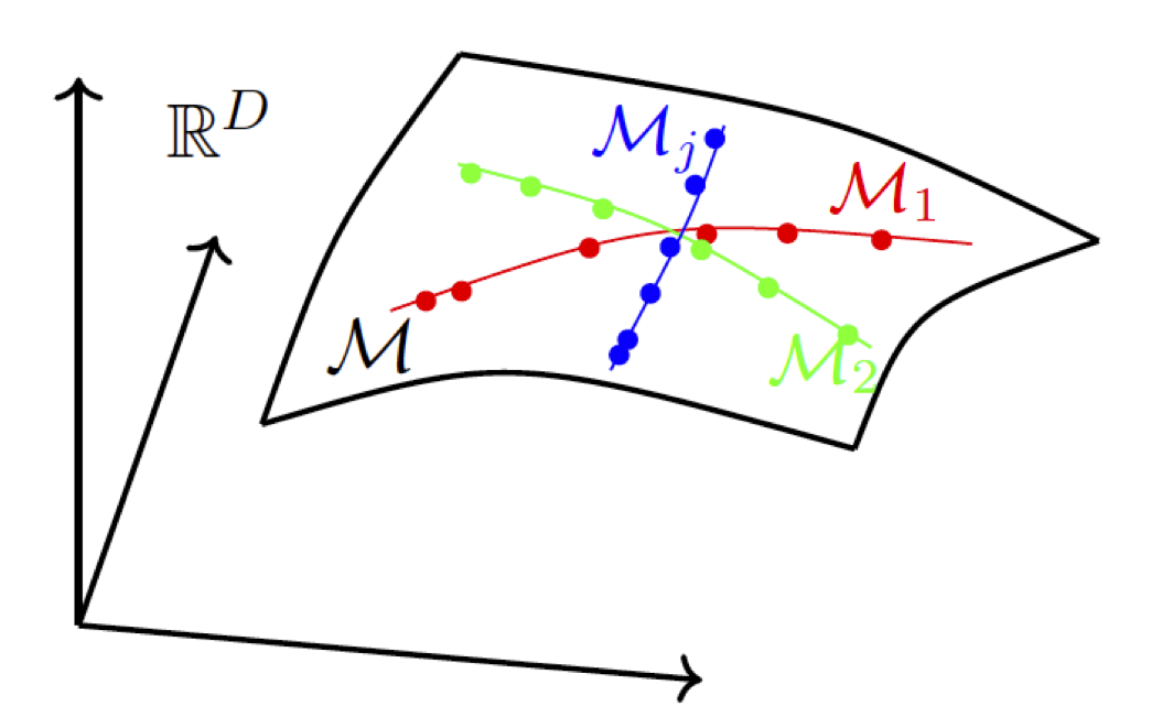
Real-world distributions typically contain multiple components or modes, for example, corresponding to different object classes in images. These modes may not be statistically independent and can even have different intrinsic dimensions. Therefore, we generally assume that the data are distributed on a mixture of low-dimensional nonlinear submanifolds embedded in a high-dimensional space. Figure 3.1 illustrates such a distribution. Another constraint is that in real-world situations we typically have access only to a finite number of samples from the data distribution, rather than prior knowledge of the exact distribution itself.
To learn such a distribution under these conditions, we must address three fundamental questions:
As we will see, the fundamental idea of compression, or dimension reduction, which we have already shown to be effective in the linear/independent case, remains a guiding principle for developing computational models and methods for general nonlinear low-dimensional distributions.
Due to its theoretical and practical importance, we examine in greater depth how this compression-based framework materializes when the distribution of interest can be well modeled or approximated by a mixture of low-dimensional subspaces or low-rank Gaussians. As later chapters show, these seemingly restrictive model classes serve as basic building blocks for algorithms that perform compression on general distributions.
In Chapter 1 we mentioned that the goal of learning is to find the simplest way to generate a given set of data. Conceptually, Kolmogorov complexity was intended to provide such a measure of complexity, but it is not computable and is not associated with any implementable scheme that can actually reproduce the data. Hence, we need an alternative, computable, and realizable measure of complexity. This leads us to the notion of entropy, introduced by Shannon in 1948 [Sha48].
To illustrate the constructive nature of entropy, let us start with the simplest case. Suppose we have a discrete random variable that takes \(N\) distinct values, or tokens, \(\{\vx _{1}, \dots , \vx _{N}\}\) with equal probability \(1/N\). We can encode each token \(\vx _{i}\) using the \(\log _{2} N\)-bit binary representation of \(i\). This coding scheme can be generalized to encoding arbitrary discrete distributions [CT91]: given a distribution \(p\) such that \(\sum _{i=1}^{N} p(\vx _{i}) = 1\), one can assign each token \(\vx _{i}\) with probability \(p(\vx _{i})\) a binary code of length \(\log _{2} [1/p(\vx _{i})] = - \log _{2} p(\vx _{i})\) bits. Hence the average number of bits, or the coding rate, needed to encode any sample from the distribution \(p(\cdot )\) is given by the expression2:
This is known as the entropy of the (discrete) distribution \(p(\cdot )\). Note that this entropy is always nonnegative and it is zero if and only if \(p(\vx _{i}) = 1\) for some \(\vx _{i}\) with \(i \in [N]\).3 For a random variable \(\vx \), we will often write \(H(\vx )\) to mean the entropy of the (marginal) distribution of \(\vx \).
When the random variable \(\vx \in \R ^{D}\) is continuous and has a probability density \(p\), one may view the limit of the above sum (3.1.1) as related to an integral:
More precisely, given a continuous probability distribution \(p\) on \(\R ^{D}\), we may discretize \(\R ^{D}\) into a union of disjoint cubes \(C_{i}^{\epsilon }\) of side length \(\epsilon ^{1/D}\), each (say) centered at \(\vx _{i}\), and define the discretized distribution \(p^{\epsilon }\) by \(p^{\epsilon }(\vx _{i}) = \Pr _{\vx \sim p}[\vx \in C_{i}^{\epsilon }]\). Then one can show that \(H(p^{\epsilon }) + \log \epsilon \approx h(p)\). By taking \(\epsilon \) to be small, we observe that the differential entropy \(h(p)\) can be negative. Interested readers may refer to [CT91] for a more detailed explanation. Similar to the discrete entropy, we will often write \(h(\vx )\) to mean the entropy of the (marginal) distribution of \(\vx \).
Example 3.1 (Entropy of Gaussian distributions). Through direct calculation, one can show that the entropy of a Gaussian random variable \(x \sim \dNorm (\mu , \sigma ^{2})\) is
Similar to the entropy of a discrete distribution, we would like the differential entropy to be associated with the coding rate of some realizable coding scheme. For example, as mentioned above, if we discretize the domain of the distribution with a grid of size \(\epsilon > 0\) with centers \(\vx _{i}\), one possible coding scheme is to map each \(\vx \) to its nearest center \(\vx _{i}\), and the entropy of the resulting discrete distribution approximates the differential entropy [CT91].
There are some caveats associated with the definition of differential entropy. For a distribution in a high-dimensional space, when its support becomes degenerate (low-dimensional), its differential entropy diverges to \(-\infty \). This fact is proved in Theorem B.1, but even in the simple explicit case of Gaussian distributions (3.1.4), when the covariance \(\vSigma \) is singular, we can see that \(\logdet (\vSigma ) = -\infty \) so we have \(h(\vx ) = -\infty \) (note that by Theorem B.1, Gaussian distributions have the largest entropy among all distributions with the same mean and covariance). In such a situation, it is not obvious how to properly quantize or encode such a distribution. Nevertheless, degenerate (Gaussian) distributions are precisely the simplest possible, and arguably the most important, instances of low-dimensional distributions in a high-dimensional space. In the next chapter, we will discuss a complete resolution to this seeming difficulty with degeneracy.
The learning problem entails recovering a (potentially continuous) distribution \(p(\vx )\) from samples \(\{\vx _{1}, \dots , \vx _{N}\}\) drawn from it. For ease of exposition, we write \(\vX = \mat {\vx _{1}, \dots , \vx _{N}} \in \R ^{D \times N}\). Because the distributions of interest are (nearly) low-dimensional, we expect their (differential) entropy to be very small. However, unlike the situations studied in the previous chapter, we do not know the family of (analytical) low-dimensional models to which \(p(\vx )\) belongs. Thus, checking whether the entropy is small seems to be the only guideline we can rely on to identify and model the distribution.
Now, given the samples alone without knowing what \(p(\vx )\) is, in theory they could be interpreted as samples from any generic distribution. In particular, they could be interpreted as any of the following:
The question is: which interpretation is better, and in what sense? Suppose that you believe these data \(\vX \) are drawn from a particular distribution \(q(\vx )\), which may be one of the above. Then we could encode the data points with the optimal codebook for the distribution \(q(\vx )\). Then, as the number of samples \(N\) becomes large, the required average coding length (or coding rate) is given by the so-called cross-entropy:
If we have identified the correct distribution \(p(\vx )\), the coding rate is given by the entropy \(h(p) = \Ex _{\vx \sim p}[-\log p(\vx )]\). It turns out that the above coding length \(\CE (p \mmid q)\) is always greater than or equal to the entropy \(h(\vx )\) unless \(p = q\).
Hence, given a set of sampled data \(\vX \), to determine which distribution best characterizes the data among \(p^{n}\), \(p^{e}\), and \(\hat {q}\), we may compare their coding rates for \(\vX \) and see which yields the lowest rate. We know from the above that the (theoretically achievable) coding rate for a distribution is closely related to its entropy. In general,
If the data \(\vX \) were encoded by the codebook associated with each of these distributions, the coding rate for \(\vX \) would therefore decrease in the same order:
This observation gives a general guideline for pursuing a distribution \(p(\vx )\) that has low-dimensional structure. It suggests two possible approaches:
Conceptually, both approaches A1 and A2 try to do the same thing. For A1, we need to ensure such a path of transformation exists and is computable. For A2, it is necessary that the chosen family is rich enough and can closely approximate (or contain) the ground-truth distribution. For either approach, we need to ensure that solutions with lower entropy or better coding rates can be efficiently computed and converge to the desired distribution quickly.4 We will explore both approaches in the remaining sections of this chapter.
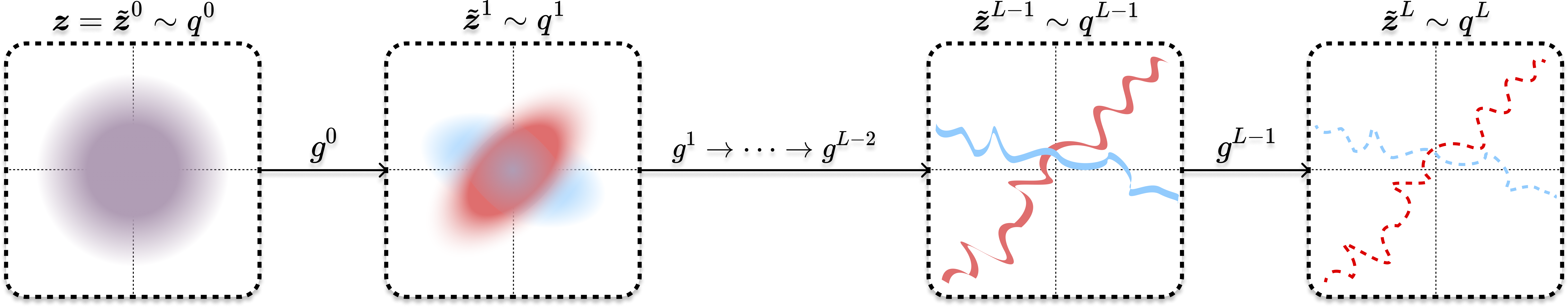
In this section we describe a natural and computationally tractable way to learn a distribution \(p_{\vx }\) by learning a parametric encoding that minimizes the entropy or coding rate of the representation, then using this encoding to transform high-entropy samples from a standard Gaussian into low-entropy samples from the target distribution, as illustrated in Figure 3.2. This methodology combines approaches A1 and A2 above to learn and sample from the distribution.
We first want a procedure that reduces the entropy of a very noisy random variable, producing a lower-entropy sample from the data distribution. Here we describe one potential approach, perhaps the most natural. First, we devise a way to gradually increase the entropy of samples already drawn from the data distribution. Next, we seek an approximate inverse of this process. In general, increasing entropy has no inverse, because information from the original distribution may be destroyed. We therefore restrict ourselves to a special case in which (1) the entropy-increasing operation is simple, computable, and reversible, and (2) we have a (parametric) encoding of the data distribution, as alluded to above. As we will see, these two conditions make our approach feasible.
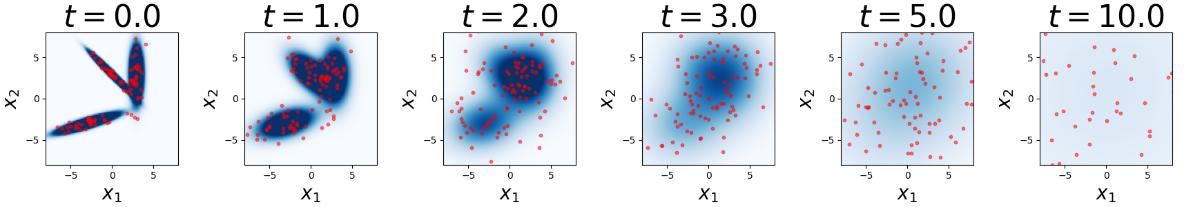
We will increase the entropy in arguably the simplest possible way, i.e., adding isotropic Gaussian noise. More precisely, given the random variable \(\vx \), we can consider the stochastic process \((\vx _{t})_{t \in [0, T]}\) that adds gradual noise to it, i.e.,
where \(T \in [0, \infty )\) is a time horizon and \(\vg \sim \dNorm (\vzero , \vI )\) is drawn independently of \(\vx \). This process is an example of a diffusion process, so named because it spreads (i.e., diffuses) the probability mass over all of \(\R ^{D}\) as time goes on, increasing the entropy. This intuition is confirmed graphically by Figure 3.3, and rigorously via the following theorem.
Theorem 3.1 (Simplified version of Theorem B.2). Suppose that \((\vx _{t})_{t \in [0, T]}\) follows the model (3.2.1). For any \(t \in (0, T]\), the random variable \(\vx _{t}\) has a probability density \(p_{t}\) and differential entropy \(h(\vx _{t}) > -\infty \). Moreover, under certain technical conditions on \(\vx \),
The proof is elementary, but it is rather long, so we postpone it to Section B.2.1. The main as-yet unstated implication of this result is that \(h(\vx _{t}) > h(\vx _{s})\) for every \(t > s \geq 0\). To see this, note that if \(s = 0\) and \(h(\vx ) = h(\vx _{0}) = -\infty \) then \(h(\vx _{t}) > -\infty \) for all \(t > 0\), so the conclusion is true; otherwise \(h(\vx _{t}) = h(\vx _{s}) + \int _{s}^{t} \bs {\frac{\mathrm{d}}{\mathrm{d}u} h(\vx _{u})} \odif {u} > h(\vx _{s})\) by the fundamental theorem of calculus, so in both cases \(h(\vx _{t}) > h(\vx _{s})\) for every \(t > s \geq 0\).
Example 3.2 (Adding noise to a mixture of Gaussians). In this example, we consider adding noise to a mixture of \(K\) Gaussians. Choose \(K\) means \(\vmu _{1}, \dots , \vmu _{K} \in \R ^{D}\), \(K\) covariance matrices \(\vSigma _{1}, \dots , \vSigma _{K} \in \PSD (D)\), and probabilities \(\pi _{1}, \dots , \pi _{K} \in [0, 1]\) such that \(\sum _{k = 1}^{K}\pi _{k} = 1\). Then \(\vx \) is sampled as follows.
Thus \(\vx \) has the Gaussian mixture distribution
The inverse operation to adding noise is known as denoising. It is a classical and well-studied topic in signal processing and system theory, instantiated (for example) as the Wiener filter and the Kalman filter (see Section 1.3.1). Several problems discussed in Chapter 2, such as PCA, ICA, and Dictionary Learning, are specific instances of the denoising problem. For a fixed \(t\) and the additive Gaussian noise model (3.2.1), the denoising problem can be formulated as attempting to learn a function \(\bar {\vx }^{\star }(t, \cdot )\) that forms the best possible approximation (in expectation) of the true random variable \(\vx \), given both \(t\) and \(\vx _{t}\):
The solution to this problem, when optimizing \(\bar {\vx }(t, \cdot )\) over all possible (square-integrable) functions, is the so-called Bayes optimal denoiser, and turns out to be the conditional expectation:
This expression justifies the notation \(\bar {\vx }\), which computes a conditional expectation (i.e., conditional mean or conditional average). In short, it attempts to remove the noise from the noisy input, outputting the best possible guess (in expectation and with respect to the \(\ell ^{2}\) distance) of the denoised original random variable.
Example 3.3 (Denoising Gaussian Noise from a Mixture of Gaussians). In this example we compute the Bayes optimal denoiser for an important class of distributions, the Gaussian mixture model in Example 3.2. Let us define \(\phi (\vx ; \vmu , \vSigma )\) as the probability density of \(\dNorm (\vmu , \vSigma )\) evaluated at \(\vx \). In this notation, the density of \(\vx _{t}\) is
Conditioned on \(y\), the variables are jointly Gaussian: if we write \(\vx = \vmu _{y} + \vSigma _{y}^{1/2}\vu \) where \((\cdot )^{1/2}\) is the matrix square root and \(\vu \sim \dNorm (\vzero , \vI )\) independently of \(y\) (and \(\vg \)), then we have
The probability can be dealt with as follows. Let \(p_{t \mid y}\) be the probability density of \(\vx _{t}\) conditioned on the value of \(y\). Then
On the other hand, the conditional expectation is as described before:
This example is particularly important, and several special cases will give us great conceptual insight later. For now, let us attempt to extract some geometric intuition from the functional form of the optimal denoiser (3.2.19).
To understand (3.2.19) intuitively, let us first set \(K = 1\) (i.e., one Gaussian) such that \(\vx \sim \dNorm (\vmu , \vSigma )\). Let us then diagonalize \(\vSigma = \vV \vLambda \vV ^{\top }\). Then the Bayes optimal denoiser is
where \(\lambda _{1}, \dots , \lambda _{D}\) are the eigenvalues of \(\vSigma \). We can observe that this denoiser has three steps:
This is the geometric interpretation of the denoiser of a single Gaussian. The overall denoiser of the Gaussian mixture model (3.2.19) uses \(K\) such denoisers, weighting their output by the posterior probabilities \(\Pr [y = k \mid \vx _{t}]\). If the means of the Gaussians are well separated, these posterior probabilities are very close to \(0\) or \(1\) near each mean or cluster. In this regime, the overall denoiser (3.2.19) has the same geometric interpretation as the above single Gaussian denoiser. \(\blacksquare \)
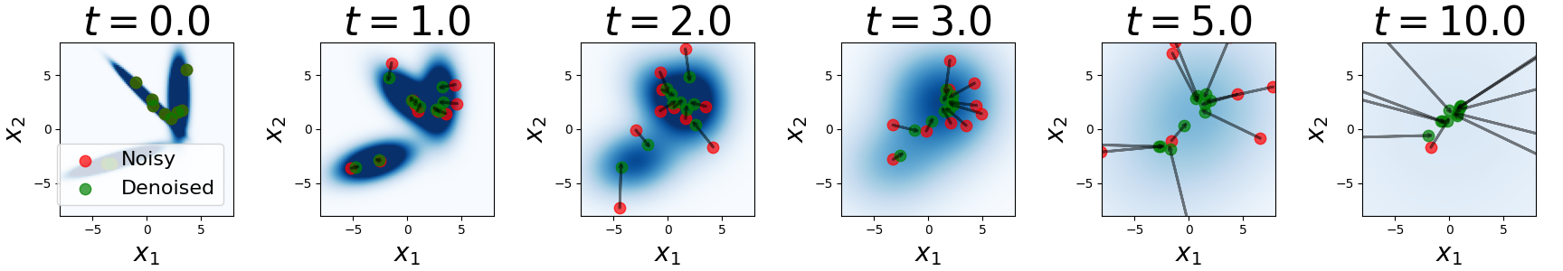
Intuitively, and as we can see from Example 3.3, the Bayes-optimal denoiser \(\bar {\vx }^{\star }(t, \cdot )\) should move its input \(\vx _{t}\) toward the modes of the distribution of \(\vx \). It turns out that we can quantify this by showing that the Bayes-optimal denoiser takes a gradient-ascent step on the (log-)density of \(\vx _{t}\), which (recall) we denoted \(p_{t}\). That is, following the denoiser means moving from the input iterate to a region of higher probability within this (perturbed) distribution. For small \(t\), the perturbation is small, so our initial intuition is therefore almost exactly right. The picture is visualized in Figure 3.4 and rigorously formulated as Tweedie’s formula [Rob56].
Theorem 3.2 (Tweedie’s Formula). Suppose that \((\vx _{t})_{t \in [0, T]}\) obeys (3.2.1). Let \(p_{t}\) be the density of \(\vx _{t}\) (as previously declared). Then
Proof. For the proof, suppose that \(\vx \) has a density,5 and call this density \(p\). Let \(p_{0 \mid t}\) and \(p_{t \mid 0}\) be the conditional densities of \(\vx = \vx _{0}\) given \(\vx _{t}\) and \(\vx _{t}\) given \(\vx \) respectively. Let \(\phi (\vx ; \vmu , \vSigma )\) be the density of \(\dNorm (\vmu , \vSigma )\) evaluated at \(\vx \), so that \(p_{t \mid 0}(\vx _{t} \mid \vx ) = \phi (\vx _{t} ; \vx , t^{2}\vI )\). Then a simple calculation gives
Simple rearrangement of the above equality proves the theorem. □
This result develops a connection between denoising and optimization: the Bayes-optimal denoiser takes a single step of gradient ascent on the perturbed data density \(p_{t}\), and the step size adaptively becomes smaller (i.e., takes more precise steps) as the perturbation to the data distribution grows smaller. The quantity \(\nabla _{\vx _{t}}\log p_{t}(\vx _{t})\) is called the (Hyvärinen) score and frequently appears in discussions about denoising, etc.; it first appeared in a paper of Aapo Hyvärinen in the context of ICA [Hyv05].
Similar to how one step of gradient descent is almost never sufficient to minimize an objective in practice when initializing far from the optimum, the output of the Bayes-optimal denoiser \(\bar {\vx }^{\star }(t, \cdot )\) is almost never contained in a high-probability region of the data distribution when \(t\) is large, especially when the data have low-dimensional structure. We illustrate this point explicitly in the following example.
Example 3.4 (Denoising a two-point mixture). Let \(x\) be uniform on the two-point set \(\{-1, +1\}\) and let \((x_{t})_{t \in [0, T]}\) follow (3.2.1). This is precisely a degenerate Gaussian mixture model with priors equal to \(\frac {1}{2}\), means \(\{-1, +1\}\), and covariances both equal to \(0\). For a fixed \(t > 0\) we can use the calculation of the Bayes-optimal denoiser in (3.2.19) to obtain (proof as exercise)
Therefore, to denoise the very noisy sample \(\vx _{T}\) (where, recall, \(T\) is the maximum time), we cannot use the denoiser just once. Instead, we must apply it many times, analogously to gradient descent with decaying step sizes, to converge to a stationary point \(\hat {\vx }\). Namely, we use the denoiser to go from \(\vx _{T}\) to \(\hat {\vx }_{T - \delta }\), which approximates \(\vx _{T - \delta }\), then from \(\hat {\vx }_{T - \delta }\) to \(\hat {\vx }_{T - 2\delta }\), and so on, all the way from \(\hat {\vx }_{\delta }\) to \(\hat {\vx } = \hat {\vx }_{0}\). Each denoising step makes the action of the denoiser more like a gradient step on the original (log-)density.
More formally, we uniformly discretize \([0, T]\) into \(L + 1\) timesteps \(0 = t_{0} < t_{1} < \cdots < t_{L} = T\), i.e.,
Then for each \(\ell \in [L] = \{1, 2, \dots , L\}\), going from \(\ell = L\) to \(\ell = 1\), we run the iteration
At the beginning of the iteration, when \(\ell \) is large, we barely trust the denoiser’s output and mostly keep the current iterate. This makes sense, as the denoiser can have huge variance (cf. Example 3.4). When \(\ell \) is small, the denoiser “locks on” to the modes of the data distribution, since a denoising step is essentially a gradient step on the true distribution’s log-density, and we can trust it not to produce unreasonable samples; thus the denoising step is dominated by the denoiser’s output. At \(\ell = 1\) we even discard the current iterate and keep only the denoiser’s output.
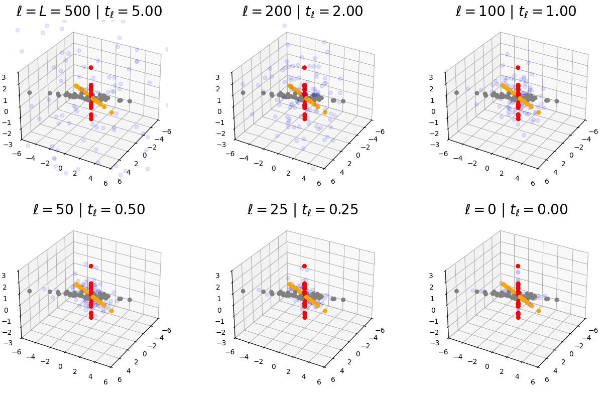
We visualize the convergence process in \(\R ^{3}\) in Figure 3.5. While we will develop some rigorous results about convergence later, we now give a closed-form example of the iterative denoising process applied to denoising a Gaussian data distribution.
Example 3.5 (Iterative denoising for a single Gaussian). To understand the above iterative denoising iteration intuitively, we apply it to denoise \(\vx _{T}\) defined in (3.2.1), where \(\vx \sim \dNorm (\vmu , \vSigma )\). Using (3.2.42), we compute
Then, plugging in the form for \(\bar {\vx }^{\star }\) that we obtain from (3.2.22) and performing some tedious matrix algebra, we obtain

Recall that we wanted to build the iterative denoising process to reduce the entropy of the iterates. While we did this in a roundabout way by inverting a process that adds entropy, it is now time to pay the piper and confirm that our iterative denoising process reduces the entropy.
Theorem 3.3 (Simplified Version of Theorem B.3). Suppose that \((\vx _{t})_{t \in [0, T]}\) obeys (3.2.1). Then, under certain technical conditions on \(\vx \), for every \(s < t\) with \(s, t \in (0, T]\),
The full statement of the theorem and the proof itself require some technicality, so they are postponed to Section B.2.2.
The last thing we discuss here is that many times, we will not be able to compute \(\bar {\vx }^{\star }(t, \cdot )\) for any \(t\), since we do not have the distribution \(p_{t}\). But we can try to learn one from data. Recall that the denoiser \(\bar {\vx }^{\star }\) is defined in (3.2.7) as minimizing the mean-squared error \(\Ex \norm {\bar {\vx }(t, \vx _{t}) - \vx }_{2}^{2}\). We can use this mean-squared error as a loss or objective function to learn the denoiser. For example, we can parameterize \(\bar {\vx }(t, \cdot )\) by a neural network, writing it as \(\bar {\vx }_{\theta }(t, \cdot )\), and optimize the loss over the parameter space \(\Theta \):
The solution to this optimization problem, implemented via gradient descent or a similar algorithm, will give us a \(\bar {\vx }_{\theta ^{\star }}(t, \cdot )\) which is a good approximation to \(\bar {\vx }^{\star }(t, \cdot )\) (at least if the training works) and which we will use as our denoiser.
What is a good architecture for this neural network \(\bar {\vx }_{\theta ^{\star }}(t, \cdot )\)? To answer this question, we will first attempt to understand the case of data \(\vx \) that are low-rank, i.e., having low-rank support. The most canonical way to represent low-rank data is through a low-rank Gaussian, and so we start our exploration by assuming that \(\vx \) is drawn (approximately) from a low-rank Gaussian:
where \(\vU \in \O (D, P)\) is a tall orthogonal matrix with \(P \leq D\) (using zero-mean for essentially notational convenience). The optimal denoiser under (3.2.50) is (from Example 3.3):
The matrix \(\vU \vU ^{\top } + t^{2}\vI \) is a low-rank perturbation of the full-rank matrix \(t^{2}\vI \), and thus ripe for simplification via the Sherman-Morrison-Woodbury identity, i.e., for matrices \(\vA , \vC , \vU , \vV \) such that \(\vA \) and \(\vC \) are invertible,
We prove this identity in Exercise 3.3. For now we apply this identity with \(\vA = t^{2}\vI \), \(\vU = \vU \), \(\vV = \vU ^{\top }\), and \(\vC = \vI \), obtaining
This implies
Our optimal denoiser is a (rescaled) linear projection onto the low-rank subspace supporting our data distribution. This is essentially the same thing as probabilistic PCA from Chapter 2 (cf. Section 2.1.4). We can formalize this intuition by considering a class of subspace-parameterized denoisers:
and showing that the denoising problem \(\min _{\vV \in \O (D, P)}\Ex \norm {\bar {\vx }_{\vV }(t, \vx _{t}) - \vx }_{2}^{2}\) obtains the same solution as probabilistic PCA (Section 2.1.4). Indeed, plugging our subspace denoiser into the training loss (3.2.7), we obtain
where the equality is due to (3.2.1). Conditioned on \(\vx \) (thus integrating over \(\vg \)), we compute
where the second equality follows from \(\vg \sim \dNorm (\vzero , \vI )\) and the fact that \(\vV \in \O (D, P)\) so that \( \Ex _{\vg }\norm {\vV \vV ^\top \vg }_{2}^{2} = \Ex _{\vg }\norm {\vV ^\top \vg }_{2}^{2} = P\). Therefore, the denoising problem is equivalent to
which in turn is equivalent to the problem
which was shown in Section 2.1.1 to be equivalent to the problem
i.e., the probabilistic PCA formulation (2.1.30).
Thus, if we were to assume our data were drawn from a low-rank Gaussian, our denoising algorithm would essentially consist of many PCA iterations in a row applied to progressively less-noisy data. While this method sounds very simple, it can actually produce complex and relatively powerful denoising behaviors when applied to practical data, as demonstrated by PCANet [CJG+15]. Nevertheless, to obtain a more general denoising operator that may work on complex and multi-modal data distributions, we will consider a broader class of data distributions: the ubiquitous class of low-rank Gaussian mixture models, whose denoiser we computed in Example 3.2 and Example 3.3. In the context of denoising, since Gaussian mixture models can approximate a very broad class of distributions arbitrarily well, in practice optimizing among the class of denoisers for Gaussian mixture models can potentially give us something close to the optimal denoiser for the real data distribution.
Formally, we now assume that \(\vx \) is drawn from a low-rank Gaussian mixture model \(\frac {1}{K}\sum _{k = 1}^{K}\dNorm (\vzero , \vU _{k}\vU _{k}^{\top })\), where \(\vU _{k} \in \O (D, P)\) are tall orthogonal matrices whose columns span the \(P\)-dimensional subspaces that support the \(K\) low-rank Gaussian components. We write
Then the optimal denoiser under (3.2.1) is (from Example 3.3)
Applying the same Sherman-Morrison-Woodbury identity as in (3.2.55), we obtain
We can then compute the posterior probabilities as follows. Since the \(\vU _{k}\) are orthogonal, \(\det (\vU _{k}\vU _{k}^{\top } + t^{2}\vI )\) is the same for every \(k\). Thus
This is a softmax operation weighted by the projection of \(\vx _{t}\) onto each subspace measured by \(\norm {\vU _{i}^{\top }\vx _{t}}_{2}\) (tempered by the temperature \(2t^{2}(1 + t^{2})\)). Meanwhile, the component denoisers can be written in the same way as (3.2.58) to obtain
Putting these together, we have
i.e., a projection of \(\vx _{t}\) onto each of the \(K\) subspaces, weighted by a softmax of a quadratic function of \(\vx _{t}\). This functional form is similar to an attention mechanism in a transformer architecture! As we will see in Chapter 5, this is no coincidence at all; the deep link between denoising and lossy compression (to be covered in Section 4.1) makes transformer denoisers so effective in practice. Thus, our Gaussian mixture model theory motivates the use of transformer-like neural networks for denoising.
Overall, the learned denoiser architecture corresponds to an (implicit parametric) encoding scheme of the given data, since it can be used to denoise/project onto the data distribution. Training a denoiser is equivalent to finding a better coding scheme, and this partially implements approach A2 (i.e., pursuing a distribution by searching for schemes with better coding rates) at the end of Section 3.1.3. In the sequel, we discuss how to implement the other approach.
Remember that at the end of Section 3.1.3, we discussed two approaches for pursuing a distribution with low-dimensional structure. The first approach (A1) starts with a normal distribution of high entropy and gradually reduces its entropy until it reaches the data distribution. We call this procedure sampling, since we generate new samples. It is now time to discuss how to implement this with the toolkit we have built.
We know how to denoise very noisy samples \(\vx _{T}\) to obtain approximations \(\hat {\vx }\) whose distributions resemble that of the target random variable \(\vx \). Yet the sampling procedure requires us to start from a template distribution that has no influence from the distribution of \(\vx \) and to use the denoiser to guide the iterates toward the distribution of \(\vx \). How can we do this? One way is motivated as follows:
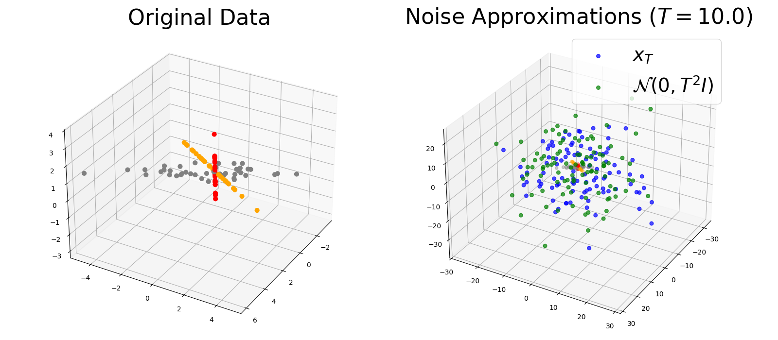
Thus, \(\vx _{T} \approx \dNorm (\vzero , T^{2}\vI )\). This approximation is quite good for almost all practical distributions, and is visualized in Figure 3.7.
So, discretizing \([0, T]\) into \(0 = t_{0} < t_{1} < \cdots < t_{L} = T\) uniformly using \(t_{\ell } = T\ell / L\) (as in the previous section), one possible way to sample from pure noise is:
Run the denoising iteration as in Section 3.2.1, i.e.,
This is conceptually all there is behind diffusion models, which transform noise into data samples in accordance with the first desideratum. However, a few steps remain before we obtain models that can actually sample from real data distributions like images under practical resource constraints. In the sequel, we introduce and motivate several such steps.
Step 1: Different discretizations. The first step is motivated by the observation that we do not need to spend so many denoising iterations at large \(t\). Figure 3.5 shows that the first \(200\) or \(300\) iterations out of the \(500\) iterations of the sampling process are spent contracting the noise toward the data distribution as a whole, before the remaining iterations push the samples toward a subspace. Given a fixed iteration count \(L\), this suggests that we should allocate more timesteps \(t_{\ell }\) near \(t = 0\) than near \(t = T\). During sampling (and training), we can therefore use an alternative discretization of \([0, T]\) into \(0 \leq t_{0} < t_{1} < \cdots < t_{L} \leq T\), such as an exponential discretization:
where \(C_{1}, C_{2} > 0\) are constants that can be tuned for optimal performance in practice; theoretical analyses often specify such optimal constants as well. The denoising/sampling iteration then becomes
with \(\hat {\vx }_{t_{L}} \sim \dNorm (\vzero , t_{L}^{2}\vI )\).
Step 2: Different noise models. The second step is to consider slightly different models compared to (3.2.1). The basic motivation for this is as follows. In practice, the noise distribution \(\dNorm (\vzero , t_{L}^{2}\vI )\) becomes an increasingly poor estimate of the true covariance in high dimensions, i.e., (3.2.81) becomes an increasingly poor approximation, especially with anisotropic high-dimensional data. The increased distance between \(\dNorm (\vzero , t_{L}^{2}\vI )\) and the true distribution of \(\vx _{t_{L}}\) may cause the denoiser to perform worse in such circumstances. Theoretically, \(\vx _{t_{L}}\) never converges to any distribution as \(t_{L}\) increases, so this setup is difficult to analyze end-to-end. In this case, our remedy is to simultaneously add noise and shrink the contribution of \(\vx \), such that \(\vx _{T}\) converges as \(T \to \infty \). The rate of added noise is denoted \(\sigma \colon [0, T] \to \R _{\geq 0}\), and the rate of shrinkage is denoted \(\alpha \colon [0, T] \to \R _{\geq 0}\), such that \(\sigma \) is increasing and \(\alpha \) is (not strictly) decreasing, and
The previous setup has \(\alpha _{t} = 1\) and \(\sigma _{t} = t\), and this is called the variance-exploding (VE) process. A popular choice that decreases the contribution of \(\vx \), as we described originally, has \(T = 1\) (so that \(t \in [0, 1]\)), \(\alpha _{t} = \sqrt {1 - t^{2}}\) and \(\sigma _{t} = t\); this is the variance-preserving (VP) process. Note that under the VP process, \(\vx _{1} \sim \dNorm (\vzero , \vI )\) exactly, so we can just sample from this standard distribution and iteratively denoise. As a result, the VP process is much easier to analyze theoretically and more stable empirically.6
With this more general setup, Tweedie’s formula (3.2.23) becomes
The denoising iteration (3.2.84) becomes
Example 3.6 (Gaussian mixture model). For a Gaussian mixture model (see Example 3.2), its denoiser (3.2.19) becomes
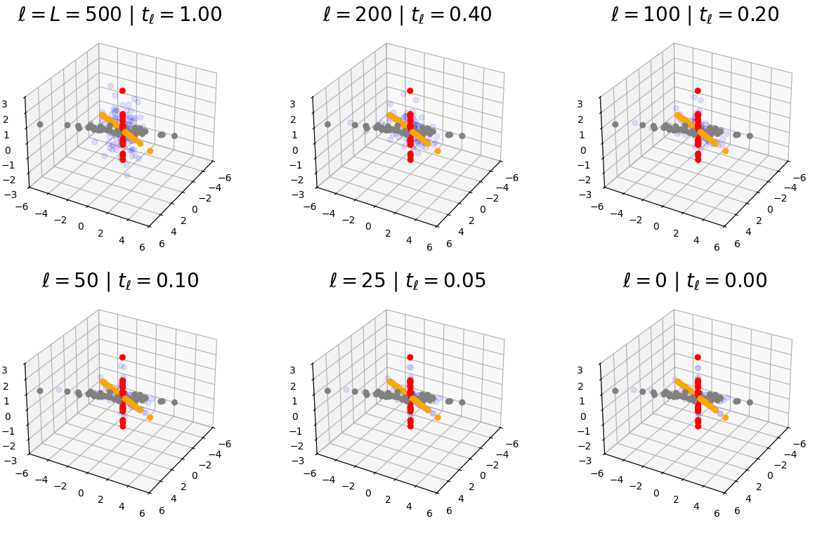
Figure 3.8 demonstrates iterations of the sampling procedure. \(\blacksquare \)
Note that the denoising iteration (3.2.87) gives a sampling algorithm called the DDIM (“Denoising Diffusion Implicit Model”) sampler [SME20], and is one of the most popular sampling algorithms used in diffusion models today. We summarize it in Algorithm 3.1.
Step 3: Optimizing training pipelines. If we use the procedure dictated by Section 3.2.1 to learn a separate denoiser \(\bar {\vx }(t, \cdot )\) for each time \(t\) to be used in the sampling algorithm, we would have to learn \(L\) separate denoisers! This is highly inefficient—the usual case is that we have to train \(L\) separate neural networks, taking up \(L\) times the training time and storage memory, and then be locked into using these timesteps for sampling forever. Instead, we can train a single neural network to denoise across all times \(t\), taking as input the continuous variables \(\vx _{t}\) and \(t\) (instead of just \(\vx _{t}\) before). Mechanically, our training loss averages over \(t\), i.e., solves the following problem:
where \(\tau \sim \dUnif ([0, T])\), i.e., is drawn uniformly from \([0, T]\). Similar to Step 1, where we used more timesteps closer to \(t = 0\) to ensure a better sampling process, we may want to ensure that the denoiser is higher quality closer to \(t = 0\), and thereby weight the loss so that \(t\) near \(0\) has higher weight.7 Letting \(w_{t}\) be the weight at time \(t\), the weighted loss would look like
One reasonable choice of weight in practice is \(w_{t} = \alpha _{t}^{2}/\sigma _{t}^{2}\). The precise reason will be covered in the next paragraph, but generally it serves to up-weight the losses corresponding to \(t\) near \(0\) while still remaining reasonably numerically stable. Also, of course, we cannot compute the expectation in practice, so we use the most straightforward Monte Carlo average to estimate it. The series of changes made here have several conceptual and computational benefits: we do not need to train multiple denoisers, we can train on one set of timesteps and sample using a subset (or others entirely), etc. The full pipeline is discussed in Algorithm 3.2. Certainly, this pipeline works in practice; we discuss some results in Sections 8.6 to 8.10.
Step 4: Changing the estimation target. It is common to instead reorient the whole denoising pipeline around noise predictors, i.e., estimates of \(\Ex [\vg \mid \vx _{t}]\). In practice, noise predictors are slightly easier to train because their output is (almost) always of comparable size to a Gaussian random variable, so training is more numerically stable, but they may require larger models since they predict a full-dimensional target instead of potentially low-dimensional data [LH25]. By (3.2.85) we have
so any predictor for \(\vx \) can be turned into a predictor for \(\vg \) using the above relation, i.e.,
and vice-versa. Thus a good network for estimating \(\bar {\vg }\) is the same as a good network for estimating \(\bar {\vx }\) plus a residual connection (as seen in, e.g., transformers). Their losses are also the same as the denoiser, up to the factor of \(\alpha _{t}/\sigma _{t}\), i.e.,
recalling that \(\tau \sim \dUnif ([0, T])\). Other targets have been proposed for different tasks, e.g., \(\Ex [\vv _{t} \mid \vx _{t}]\) where \(\vv _{t} = \frac{\mathrm{d}}{\mathrm{d}t} \vx _{t}\) (called \(v\)-prediction or velocity prediction), etc. This turns out to be equivalent to denoising and noise prediction, but also fundamentally useful for generalizations of diffusion such as flow matching, which we will discuss in Remark 3.3.
We have made many changes to our original platonic noising/denoising process. To assure ourselves that the new process still works in practice, we can compute numerical examples (such as Figure 3.8). To assure ourselves that it is theoretically sound, we can prove a bound on the error rate for the sampling algorithm, which shows that the error rate is small. We now furnish such a rate from the literature, which shows that the output distribution of the sampler converges in the so-called total variation (TV) distance to the true distribution. The TV distance between two random variables \(\vx \) and \(\vy \) is defined as:8
If \(\vx \) and \(\vy \) are very close (uniformly), then the supremum will be small. So the TV distance measures the closeness of random variables. (It is indeed a metric, as the name suggests; the proof is an exercise.)
Theorem 3.4 ([LY24] Theorem 1, Simplified). Suppose that \(\Ex \norm {\vx }_{2} < \infty \). If \(\vx \) is denoised according to the VP process with an exponential discretization9 as in (3.2.83), the output \(\hat {\vx }\) of Algorithm 3.1 satisfies the total variation bound
where \(\bar {\vx }^{\star }\) is the Bayes optimal denoiser for \(\vx \), and \(\tilde {\cO }\) is a version of the big-\(\cO \) notation that ignores logarithmic factors in \(L\).
The very high-level proof technique is, as discussed earlier, to bound the error at each step, distinguish the error sources (between discretization and denoiser error), and carefully ensure that the errors do not accumulate too much (or even cancel out).
Note that if \(L \to \infty \) and we correctly learn the Bayes-optimal denoiser \(\bar {\vx } = \bar {\vx }^{\star }\) (so the excess error is \(0\)), then the sampling process in Algorithm 3.1 yields a perfect (in distribution) inverse of the noising process, since the error rate in Theorem 3.4 goes to \(0\),10 as argued heuristically above.
Remark 3.1. What if the data is low-dimensional, say supported on a low-rank subspace of the high-dimensional space \(\R ^{D}\)? If the data distribution is compactly supported—say if the data is normalized to the unit hypercube, which is often ensured as a preprocessing step for real data such as images—it is possible to do better. Namely, the authors of [LY24] also define a measure of approximate intrinsic dimension \(\kappa \) using the asymptotics of the so-called covering number, which is extremely similar in intuition (if not in implementation) to the rate-distortion function presented in the next Chapter. Then they show that using a particular small modification of the DDIM sampler in Algorithm 3.1 (i.e., slightly perturbing the update coefficients), the discretization error becomes \(\tilde {\cO }(\kappa /L)\) instead of \(\tilde {\cO }(D/L)\) as in Theorem 3.4. Therefore, using this modified algorithm, \(L\) does not have to be too large even as \(D\) reaches the thousands or millions, since real data have low-dimensional structure. However, in practice we use the DDIM sampler instead, so \(L\) should have a mild dependence on \(D\) to achieve consistent error rates. The exact choice of \(L\) trades off between the computational complexity (e.g., runtime or memory consumption) of sampling and the statistical complexity of learning a denoiser for low-dimensional structures. The value of \(L\) is often different at training time (where a larger \(L\) allows better coverage of the interval \([0, T]\), which helps the network learn a relationship that generalizes over \(t\)) and sampling time (where \(L\) being smaller means more efficient sampling). One can even pick the timesteps adaptively at sampling time to optimize this tradeoff [BLZ+22].
Remark 3.2. Various other works define the reverse process as moving backward in the time index \(t\) using an explicit difference equation, or differential equation in the limit \(L \to \infty \), or forward in time using the transformation \(\vy _{t} = \vx _{T - t}\), such that if \(t\) increases then \(\vy _{t}\) becomes closer to \(\vx _{0}\). Each paper uses its own notation, and it can sometimes be confusing to understand the relationships between different papers’ results. In this work we strive to keep consistency: we move forward in time to noise, and backward in time to denoise. If you are reading another work that is not clear on the time index, or trying to implement an algorithm that is similarly unclear, there is one way to disambiguate every time: the sampling process should always have a positive coefficient on the denoiser term (or equivalently the score function) when taking a step.
Remark 3.3. The diffusion/denoising processes and associated models provide a way to transport the data distribution to and from a high-entropy (Gaussian or Gaussian-like) distribution. On the other hand, it may be useful to transport the data distribution to and from an arbitrary target distribution, which could be Gaussian, a Gaussian mixture, or even another type of data distribution. If we have this desideratum, we can use the flow matching framework to achieve this. Suppose the target random variable is \(\vy \), and our flow is
In practice, inspired by the concept of learning a so-called transport map between data pairs \(\vx \) and \(\vy \), practitioners often wish to train a velocity predictor \(\bar {\vv }_{\theta }\) to predict \(\vv _{t} = \frac{\mathrm{d}}{\mathrm{d}t} \vx _{t} = \alpha _{t}^{\prime }\vx + \sigma _{t}^{\prime }\vy \) instead of a denoiser \(\bar {\vx }_{\theta }\), or rather train \(\bar {\vv }_{\theta }\) to predict \(\Ex [\vv _{t} \mid \vx _{t}]\). In this case, it is simplest to take the choice of coefficients \(\alpha _{t} = 1 - t\) and \(\sigma _{t} = t\) (for \(t \in [0, 1]\)), so that the prediction target is \(\vv _{t} = \vy - \vx \) for each time \(t\). Given the estimator \(\bar {\vv }_{\theta }\), the standard sampling algorithm follows the field backwards in time, i.e., starting from a realization of \(\vy \), we can iteratively update the iterate as follows:
Remark 3.4. In practice, diffusion usually takes many steps and many function evaluations of the denoiser. It is therefore natural to ask: “can we speed up the sampling process by using a smaller number of steps and function evaluations?” The answer is yes, and such models are often called consistency models or, more descriptively, few-step models. The core idea is to use a denoiser that takes in two times \(\bar {\vx }_{\theta }(s, t, \vx _{t})\) and estimates \(\Ex [\vx _{s} \mid \vx _{t}]\), which in some sense is an easier task, or alternatively to use a velocity predictor \(\bar {\vv }_{\theta }(s, t, \vx _{t})\) and estimate the average velocity \(\Ex [(\vx _{t} - \vx _{s})/(t - s) \mid \vx _{t}]\). Such denoisers have additional consistency conditions such as \(\bar {\vx }_{\theta }(u, t, \bar {\vx }_{\theta }(s, u, \vxi )) = \bar {\vx }_{\theta }(s, t, \vxi )\), which motivate auxiliary training losses. Once such a predictor is learned, the sampling process becomes very simple and efficient, as it only requires a few steps of the form
The calculation presented at the end of Section 3.2.1 seems to suggest (loosely speaking) that in practice, using a transformer-like network is a good choice for learning or approximating a denoiser. This is reasonable, but what is the problem with using any old neural network (such as a multi-layer perceptron (MLP)) and simply scaling it up to infinity? To answer this question, let us consider a constraint we have ignored or glossed over so far in this Chapter: we only have finite data with which to learn the denoiser. Indeed, let us consider the training problem (3.2.90), except this time we assume that our data \(\vx \) are drawn from the empirical distribution \(p^{\vX }\) on \(N\) training samples \(\vX = [\vx ^{(1)}, \dots , \vx ^{(N)}]\). Because \(p^{\vX }\) is supported on a \(0\)-dimensional subset of the ambient space \(\R ^{D}\), we have that \(h(p^{\vX }) = -\infty \), so in some sense \(p^{\vX }\) is the simplest (i.e., lowest-entropy) distribution that could generate our observations \(\vX \). In short, this assumption arguably has the least inductive bias about the data distribution! Many popular commentaries on deep learning and generative models would have you believe that, due to this property, the best way to solve the generative modeling problem is to scale a generic denoiser as large as possible and reap the corresponding benefits. However, this advice is (provably!) wrong in this setting. To understand why, let us note that the empirical distribution \(p^{\vX }\) is actually a mixture of Gaussians with zero covariances:
As such, we know that the (globally) optimal solution to the denoising problem (3.2.90) with \(\vx \) drawn from the empirical distribution, written out as follows:
where \(\vx _{t}^{(i)}\) is the noised version of the training sample \(\vx ^{(i)}\). The optimizer of this loss over all (square-integrable) denoisers \(\bar {\vx }\) is the associated optimal Gaussian denoiser from Example 3.3, i.e.,
This is a convex combination of the data \(\vx ^{(i)}\), and the coefficients get “sharper” (i.e., closer to \(0\) or \(1\)) as \(t \to 0\). In particular, for small \(t\), the denoiser is almost exactly equal to the closest sample in the training set, and the update moves the iterate closer to the closest point, such that at the end of sampling, the iterate \(\hat {\vx }\) is (nearly) equal to a training sample \(\vx ^{(i)}\). Let us re-emphasize this point: if we use the denoiser (3.3.3) and a good sampler, our samples will re-generate the training data. This is confirmed by our theoretical guarantee on sampling Theorem 3.4, which, when instantiated in this context, says that if we take the number of sampling steps to \(\infty \) and use the prescribed timestep schedule, the diffusion model associated with the denoiser (3.3.3) will always sample from the empirical distribution and thus always reproduce a training sample. This phenomenon is a particularly strict instantiation of memorization in generative modeling.11
Since in practice we only have a fixed finite dataset on which we can train our denoiser, the learning problem we aim to solve in this case is the finite-sample denoising loss (3.3.2) (compared to the infinite-sample denoising loss (3.2.90), for example). As such, if we have an arbitrarily large model and optimize it as well as possible, it will learn to memorize and re-generate the training set. In other words, this very large-scale model is not much more interesting than a simple database of the training data.
The above argument holds for arbitrarily powerful models that can fit the (true) memorizing denoiser. It is therefore relevant to ask whether it actually bears out in practice: do very large models (relative to the dataset) learn to memorize the training data? It turns out that this is empirically true. One of the first studies on this was [YCK+23]. To understand their results, we define the memorization ratio as the probability of memorization:
where \(\mathrm {DM}(\bar {\vx })\) is the distribution induced by the diffusion model that uses denoiser \(\bar {\vx }\), and the sample \(\hat {\vx }\) is memorized using the following criterion:
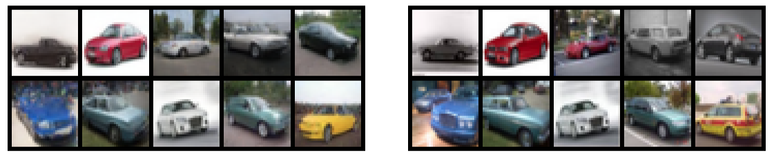
where \(\vx _{(i)}(\hat {\vx })\) is the \(i\th \) closest point to \(\hat {\vx }\) in the training dataset (in the Euclidean norm), and \(1/3\) is a constant that is empirically shown to agree well with human perception of memorization. Notice that this definition exactly corresponds to our earlier intuitive definition of memorization as sampled points each being much closer to a particular training sample than all other training samples. They showed that this kind of memorization occurs in practice when the model is much larger (in terms of the number of parameters) relative to the data; Figure 3.9 demonstrates that in this case, generated samples are essentially pixel-perfect copies of training samples. Slightly later, [GDP+23] performed a careful study to characterize how various factors such as architectures and training time impact memorization, showing among other things that as the dataset size increases relative to a fixed model, the memorization ratio rapidly changes from near-1 to near-0, i.e., the model quickly stops memorizing. This indicates the possibility of a phase transition between memorization and generalization as the model becomes smaller relative to the data. [BPM+25] investigates the existence and theoretical mechanism of this phase transition in synthetic data drawn from a Gaussian mixture model, demonstrating that it exists and providing a partial characterization of the model size at which models will start or stop memorizing. Other theoretical work such as [GVM25; KG24; NZM+24; ZLL+25] also attempts to provide a theoretical characterization of the phase transition in terms of model and dataset size in different settings.
In order to empirically prove the existence of a phase transition between memorization and generalization in real data, [ZZL+24] rethought the definition of memorization using the following reasoning. In the very high-dimensional space of natural images, Euclidean distances between points become much more strict [WM22], in the sense that if two images are not pixel-perfect matches to each other, then their Euclidean distances will concentrate sharply around a fixed value (scaling with the images’ dimension). This does not catch the case where certain concepts (such as copyrighted cartoon characters) are generated in novel positions, making it very difficult to form effective and practical memorization criteria around the Euclidean distance. To fix this, [ZZL+24] uses a particular function \(f_{\mathrm {SSCD}}\) (a pre-trained neural network called a Self-Supervised Copy Detector [PRR+22]) to map images into a Euclidean space, then takes the normalized inner product to obtain their (cosine) similarity, such that images that are similar due to this cosine similarity are claimed to be conceptually similar in the sense needed for memorization. Then, [ZZL+24] says that a sample \(\hat {\vx }\) is memorized if its similarity with any training point is \(> 3/5\), i.e.,
Figure 3.11 shows the outcome of taking many (around 10,000) samples from diffusion models trained on differently-sized training datasets in terms of estimating memorization and computing the training loss. The outcome is in line with the above discussion; when the model is too large relative to the training data and the training loss is too small, memorization occurs and samples reproduce the training data. Thus, our intuition applies in practice: for generative diffusion models, scaling the model is not all you need!
So now the question is: what kind of denoiser should we use? The key is to choose a network architecture that can approximate the true denoiser (say, the one corresponding to a low-rank distribution as in (3.2.80)) without approximating the memorizing denoiser (3.3.3). Some work has explored this fine line and why modern diffusion models, which use Transformer- and convolution-based architectures, can memorize and generalize in different regimes [KG24; NZM+24; ZLL+25].
Let us at last return to the initial premise of this Chapter, described in Section 3.1.3: finding the minimal-entropy distribution that models the data is the only way to learn the distribution. The above discussion has hopefully shown that this claim is false. However, a related claim, also argued in Section 3.1.3 because of its equivalence in the situations we had then considered, might still be true: finding the distribution with minimal coding rate is a way to learn the distribution. Supposing for the moment that \(\vx \) has a density \(p\), the coding rate (i.e., cross-entropy) of the empirical distribution \(p^{\vX }\) with respect to \(p\) is \(\CE (p \mmid p^{\vX }) = \infty \). This coding rate is obviously not minimal in any sense; if we use the same successively better approximations \(p^{n}\), \(p^{e}\), and \(\hat {q}\) discussed in Section 3.1.3, it holds
Minimizing the coding rate therefore seems a sensible way to learn the distribution while avoiding this issue. However, a problem of tractability now arises: how can we devise algorithms that learn the distribution by minimizing the coding rate while avoiding the drawbacks associated with overly minimizing entropy?
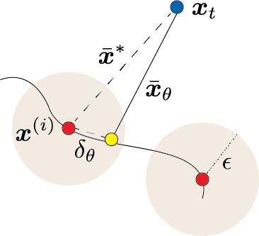
One clue is to examine what happens with successfully trained diffusion models that do not memorize. By writing the trained denoiser \(\bar {\vx }_{\theta }\) as a perturbation of the memorizing denoiser \(\bar {\vx }^{\star }\), i.e.,
we can gain graphical intuition about the action of a well-trained denoiser, as in Figure 3.12. At a very high level, the trained denoiser computes the memorizing denoiser plus some perturbation. At a small time \(t\) (perhaps even at the last step of denoising), the memorizing denoiser points entirely in the direction of a single training sample (the training sample to be re-generated by the current iterate). The distribution being learned, or denoised against, is just the empirical distribution with some \(\epsilon \)-balls around each point,12 where \(\epsilon \) is an upper bound on the magnitude of the perturbation, visualized in Figure 3.12 by the faint orange balls.13 For increasingly larger well-trained diffusion models, the perturbation radius \(\epsilon \) shrinks to \(0\), and the model learns the empirical distribution. On the other hand, \(\epsilon \) large enough that balls corresponding to different points overlap or are close may imply that the diffusion model generalizes.
Thus, our successful diffusion model can be viewed as minimizing a lossy coding rate, i.e., coding rate up to a precision \(\epsilon \) (so as to be able to disregard the \(\epsilon \)-balls around each point). This notion of the lossy coding rate turns out to be the right thing to minimize, morally speaking, and will be extremely useful. We will tease out its uses in Chapter 4 and throughout the rest of this book.
Key messages. In this Chapter, we have shown that, to pursue a general low-dimensional distribution, a universal computational approach is to start with a generic distribution and compress it toward the distribution through (iterative) noise or entropy reduction. As we discussed in the preceding Chapter, this is even the case for arguably the simplest distributions of a single subspace, such as computing PCA via the power-iteration algorithm. As we will see in future chapters, the fundamental roles of modern deep networks are not to fit arbitrary (noisy) data distributions or functions; instead, they are to realize or approximate those (lossy) compressing or denoising operators. We will derive precise forms of those operators and the associated deep architectures in future chapters.
More extensions and references. The use of denoising and diffusion for sampling has a rich history. The first work clearly about a diffusion model is probably [SWM+15], but before this there are many works on denoising as a computational and statistical problem. The most relevant of these is probably [Hyv05], which explicitly uses the score function to denoise and to perform independent component analysis. The most popular follow-ups are essentially co-occurring: [HJA20; SE19]. Since then, thousands of papers have built on diffusion models; we revisit this topic in Chapter 6.
Many of these works use a different stochastic process than the simple linear combination (3.2.85). In fact, all works listed above emphasize the need to add independent Gaussian noise at the beginning of each step of the forward process. Theoretically-minded work uses Brownian motion or stochastic differential equations to formulate the forward process [SSK+21]. However, since linear combinations of Gaussians still result in Gaussians, the marginal distributions of such processes still take the form of (3.2.85). Most of our discussion requires only that the marginal distributions are what they are, so our overly simplistic model is actually enough for almost everything. The only time marginal distributions are not enough is when we derive an expression for \(\Ex [\vx _{s} \mid \vx _{t}]\) in terms of \(\Ex [\vx \mid \vx _{t}]\). Different (noising) processes give different such expressions, which can be used for sampling (and of course there are other ways to derive efficient samplers, such as the ever-popular DDPM sampler). The process in (3.2.85) is a bona fide stochastic process whose “natural” denoising iteration takes the form of the popular DDIM algorithm [SME20]. (Even this equivalence is not trivial; we cite [DGG+25] as justification.)
On top of the theoretical work [LY24] covered in Section 3.2.2, and the lineage of work that it builds on, which studies the sampling efficiency of diffusion models when the data has low-dimensional structure, there is a large body of work that studies the training efficiency of diffusion models when the data has low-dimensional structure. Specifically, Chen et al. [CHZ+23] and Wang et al. [WZZ+24] characterized the approximation and estimation error of denoisers when the data belongs to a mixture of low-rank Gaussians, showing that the number of training samples required to accurately learn the distribution scales with the intrinsic dimension of the data rather than the ambient dimension. There is considerable methodological work that attempts to use the low-dimensional structure of the data to perform various tasks with diffusion models. We highlight three: image editing [CZG+24], watermarking [LZQ24], and unlearning [CZL+25], though this list is inexhaustive.
Exercise 3.2. Consider random vectors \(\vx \in \bR ^D\) and \(\vy \in \bR ^d\), such that the pair \((\vx , \vy ) \in \bR ^{D + d}\) is jointly Gaussian. This means that
In this exercise, we will prove that the conditional distribution \(p_{\vx \mid \vy }\) is Gaussian: namely,
where \(\vm = \vmu _{\vx } + \vSigma _{\vx \vy }\vSigma _{\vy }^{-1}(\vy - \vmu _{\vy })\).
Exercise 3.3. Show the Sherman–Morrison–Woodbury identity, i.e., for matrices \(\vA \), \(\vC \), \(\vU \), \(\vV \) such that \(\vA \), \(\vC \), and \(\vA + \vU \vC \vV \) are invertible,
Exercise 3.4. Rederive the following, assuming \(\vx _{t}\) follows the generalized noise model (3.2.85).
Exercise 3.6. Consider the somewhat familiar interpolation