“Everything should be made as simple as possible, but not any simpler.”
\(~\) – Albert Einstein
In the past chapters, we have argued that the fundamental goal of learning is to identify a data distribution with low-dimensional support and transform it into a compact and structured representation. This entails two related problems:
In Chapters 3 and 4, we have developed a complete computational solution to the distribution learning problem for general data distributions, based on the diffusion-denoising process. In Chapter 4, we have defined a compression-based objective function, the information gain, whose maximization leads to compact and structured representations. And in Chapter 5, we have seen that the layers of popular deep network architectures can be interpreted as incremental optimization steps towards maximizing the information gain. This leaves us poised to present a mathematically-founded solution to the representation learning problem.
However, when we try to achieve a certain objective through optimization, there is no guarantee that the solution \(\Z \) found in the end by greedy optimization is the correct solution. In fact, even if the optimization process manages to find the globally optimal solution \(\Z ^*\), there is no guarantee that the solution corresponds to a complete representation of the data distribution.1 Therefore, an outstanding question is: how can we ensure that the learned representation of the data distribution is correct or good enough?
Of course, the only way to verify this is to see whether there exists a decoding map, say \(g\), that can decode the learned representation to reproduce the original data (distribution) well enough:
in terms of some measure of similarity:
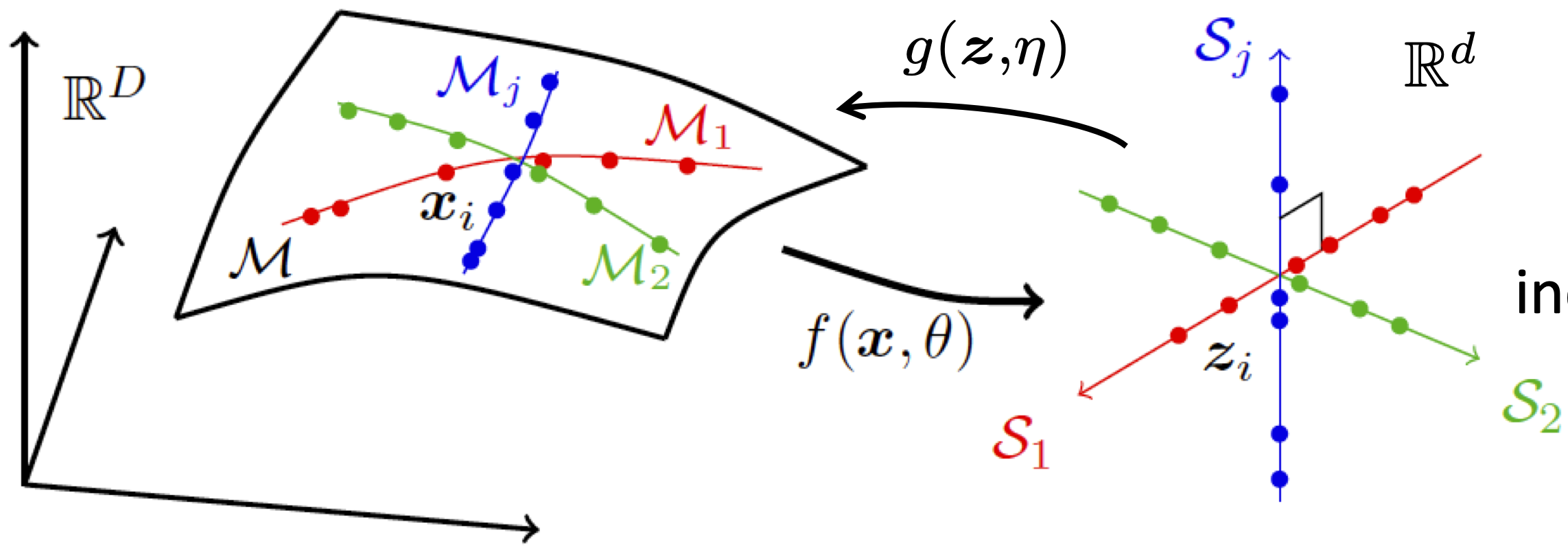
This leads to the concept of consistent representation.2 As we have briefly alluded to in Chapter 1 (see Figure 1.25), autoencoding, which integrates the encoding and decoding processes, is a natural framework for learning such a representation. We have studied some important special cases in Chapter 2 where the supports of the distribution are piecewise linear. In this chapter, Section 6.1, we will study how to extend autoencoding to more general classes of distributions whose supports are nonlinear, as illustrated in Figure 6.1, while enforcing the consistency between \(\X \) and \(\hat \X \).
Given this classical autoencoding formalism, there is a natural question: where does distribution learning end and representation learning begin? As we will see, the answer comes down to efficiency. It is typically far more effective, as demonstrated by modern practice, to learn a compact representation for the data distribution as a type of ‘preparation’ of the distribution, and only then to perform distribution learning on the so-learned representation. This is the dominant methodology in practical problems. We will demonstrate the links between the foundations we have developed in Chapters 4 and 5 and the state of the art in Section 6.1.5, where the “representation autoencoder” framework demonstrates how open-loop learned representations (which we discussed in Section 4.3.2, and will review) can be combined with a simple decoder and a \(\vZ \)-space diffusion process to enable efficient, simultaneous representation learning and sampling.
More fundamentally, in many practical and natural learning scenarios, it can be difficult or even impossible to compare distributions of the data \(\X \) and \(\hat \X \). We are left with the only option of comparing the learned feature \(\Z \) with its image \(\hat \Z \) under the encoder \(f\):
This leads to the notion of a self-consistent representation. In Section 6.2, we will study when and how we can learn a consistent representation by enforcing the self-consistency between \(\Z \) and \(\hat \Z \) only through a closed-loop transcription framework.
Furthermore, in many practical and natural learning scenarios, we normally do not have sufficient samples of the data distribution all available at once. For example, animals and humans develop their visual memory by continuously taking in increments of observations throughout their lives. In Section 6.3, we will study how to extend the closed-loop transcription framework to learn a self-consistent representation in a continuous learning setting.
Of course, a fundamental motivation for why we ever want to identify the low-dimensional structures in a data distribution and find a good representation is to make it easy to use the data for various tasks of intelligence, such as classification, completion, and prediction. Therefore, the resulting joint representation \((\x , \z )\) must be structured in such a way that is best suited for these tasks. In the following chapter, we will see how the learned representation can be structured to facilitate conditioned completion or generation tasks.
Here we give a formal definition of consistent representations, which are closely related to the concept of autoencoding.
Definition 6.1 (Consistent Representations). Given data \(\vX \), a consistent representation is a pair of functions \((f \colon \cX \to \cZ , g \colon \cZ \to \cX )\), such that the features \(\vZ = f(\vX )\) are compact and structured, and the autoencoding
Astute readers may have noticed that if we do not impose certain requirements on the representation \(\Z \) sought, the above problem has a trivial solution: one may simply choose the functions \(f\) and \(g\) to be the identity map! Hence, the true purpose of seeking an autoencoding is to ensure that the \(\Z \) so obtained is both more compact and more structured than \(\X \). As we have seen in Chapter 5, it suffices to design the representation to maximize the rate reduction
From the definition of consistent representation, it is required that the representation \(\Z \) be sufficient to recover the original data distribution \(\X \) to some degree of accuracy. For sample-wise consistency, a typical choice is to minimize the expected reconstruction error:
For consistency in distribution, a typical choice is to minimize a certain distributional distance such as the KL divergence3:
Hence, computation aside, when we seek a good autoencoding for a data distribution \(\X \), conceptually we try to find an encoder \(f\) and decoder \(g\) such that
Notice that the quantization error \(\epsilon \) plays the role of the tradeoff parameter in this Lagrangian relaxation.
In the remainder of this section, we will study how to solve such autoencoding problems under different conditions, from simple and ideal cases to increasingly more challenging and realistic conditions. We will culminate with an efficient instantiation of (6.1.5) (in Section 6.1.5) that ensures the representation space \(\vZ \) is compact and structured while also allowing for accurate reconstruction and efficient sampling.
According to [Bal11], the phrase “autoencoder” was first introduced by Hinton and Rumelhart [RHW86a] so that a deep representation could be learned via back propagation (BP) in a self-supervised fashion—reconstructing the original data is the self-supervising task. However, the very same concept of seeking a compact and consistent representation has its roots in many classic studies. As we have already seen in Chapter 2, the classical PCA, ICA, and sparse dictionary learning all share a similar goal. The only difference is that when the underlying data distribution is simple (linear and independent), the encoding or decoding mappings become easy to represent and learn: they do not need to be deep and often can be computed in closed form or with an explicit algorithm.
It is instructive to see how the notion of consistency we have defined plays out in the simple case of PCA: here, the consistent encoding and decoding mappings are given by a single-layer linear transform:
where \(\vU \in \mathbb {R}^{D\times d}\) typically with \(d\ll D\). Hence \(\vU ^\top \) represents a projection from a higher-dimensional space \(\mathbb {R}^{D}\) to a lower one \(\mathbb {R}^{d}\), as illustrated in Figure 6.2.
As we saw in Chapter 2, when the distribution of \(\vx \) is indeed supported on a low-dimensional subspace \(\vU _o\), the compactness of the representation \(\vz \) produced by \(\mathcal {E}\) is a direct consequence of correctly estimating (and enforcing) the dimension of this subspace. Recall that gradient descent on the reconstruction criterion exactly yields these sample-wise consistent mappings: indeed, the optimal solution to the problem
precisely coincides with \(\vU _o\) when the dimension of the representation is sufficiently large. In this case, we obtain sample-wise consistency for free, since this guarantees that \(\vU _o\vU _o^\top \vx = \vx \). Notice that in the case of PCA, the rate reduction term in (6.1.5) becomes void as the regularization on the representation \(\Z \) sought is explicit: It spans the entire subspace of lower dimension4.
Of course, one should expect that things will no longer be so simple when we deal with more complex distributions whose underlying low-dimensional structures are nonlinear.
Data on a Nonlinear Submanifold. So, to move beyond the linear structure addressed by PCA, we may assume that the data distribution lies on a (smooth) submanifold \(\mathcal {M}\). The intrinsic dimension of the submanifold, say \(d\), is typically much lower than the dimension of the ambient space \(\mathbb {R}^D\). From this geometric perspective, we typically want to find a nonlinear mapping \(f\) such that the resulting manifold \(f(\mathcal {M})\) is flattened, as illustrated by the example shown in Figure 6.3. The resulting feature \(\vz \)-space is typically more compact (of lower-dimension) than the \(\vx \)-space, and the manifold is flat. From the statistical perspective, which is complementary to the geometric perspective but distinct in general, we may also want to ensure that the data distribution on \(\mathcal {M}\) is mapped to a sufficiently regular distribution, say a Gaussian or uniform distribution (with very low-dimensional support), in the \(\vz \)-space. In general, the problem of learning such an autoencoding mapping for this class of data distributions is known as nonlinear principal component analysis (NLPCA).
A Classical Attempt via a Two-Layer Network. As we have seen above, in the case of PCA, a single-layer linear neural network is sufficient. That is no longer the case for NLPCA. In 1991, Kramer [Kra91] proposed to solve NLPCA by using a two-layer neural network to represent the encoder mapping \(f\) (or its inverse \(g\)) based on the universal representation property of two-layer networks with sigmoid activation:
where \(\sigma (\spcdot )\) is the sigmoid function:
Cybenko [Cyb89] showed that functions of the above form (with enough hidden nodes) can approximate any smooth nonlinear function, say the encoder \(f(\spcdot )\), to an arbitrary precision. In particular, they can represent the flattening and reconstruction maps for data distributions supported on unions of low-dimensional manifolds, as in Figure 6.3. The overall architecture of the original networks proposed by Kramer is illustrated in Figure 6.4.
Unfortunately, unlike the case of PCA above, there is in general no closed-form learning scheme for the parameters \(\bm \theta = (\vW , \vb )\) of these networks. Hence it was proposed to train the network via back propagation with the supervision of reconstruction error:
Compared to the simple case of PCA, we utilize the same reconstruction objective for learning, but a far more complex nonlinear class of models for parameterizing and learning the encoder and decoder. Although universal approximation properties such as Cybenko’s suggest that in principle learning consistent autoencoders via this framework is possible—because for any random sample of data, given enough parameters, such autoencoding pairs exist—one often finds it highly nontrivial to find them using gradient descent. Moreover, to obtain a sufficiently informative reconstruction objective and model for the distribution of high-dimensional real-world data such as images, the required number of samples and hidden nodes can be huge. In addition, as a measure of the compactness of the learned representation, the (lower) dimension of \(\z \) for the bottleneck layer is often chosen heuristically.5
Manifold Flattening via a Deeper Network. Based on the modern practice of deep networks, such classical shallow and wide network architectures are known to be rather difficult to train effectively and efficiently via back propagation (BP), partly due to the vanishing gradient of the sigmoid function. Hence, the modern practice normally suggests further decomposing the nonlinear transform \(f\) (or \(g\)) into a composition of many more layers of simpler transforms, resulting in a deeper network architecture [HS06], as illustrated in Figure 6.5.
In light of universal approximation theorems such as Cybenko’s, one may initially wonder why, conceptually, deeper autoencoders should be preferred over shallow ones. From purely an expressivity perspective, we can understand this phenomenon through a geometric angle related to the task of flattening the nonlinear manifold on which our hypothesized data distribution is supported. A purely constructive approach to flattening the manifold proceeds incrementally, in parallel to what we have seen in Chapters 3 to 5 with the interaction between diffusion, denoising, and compression. In the geometric setting, the incremental flattening process corresponding to \(f_{\ell }\) takes the form of transforming a neighborhood of one point of the manifold to be closer to a flat manifold (i.e., a subspace), and enforcing local consistency with the rest of the data samples; the corresponding incremental operation in the decoder, \(g_{\ell }\), undoes this transformation. This procedure precisely incorporates curvature information about the underlying manifold, which is estimated from data samples. Given enough samples from the manifold and a careful instantiation of this conceptual process, it is possible to implement this sketch as a computational procedure that verifiably flattens nonlinear manifolds in a white-box fashion [PPR+24]. However, the approach is limited in its applicability to high-dimensional data distributions such as images due to unfavorable scalability, motivating the development of more flexible methods for incremental autoencoding.
In the above autoencoding schemes, the dimension of the feature space \(d\) is typically chosen to be much lower than that of the original data space \(D\) in order to explicitly enforce or promote the learned representation to be low-dimensional. However, in practice, we normally do not know the intrinsic dimension of the data distribution. Hence, the choice of the feature space dimension for autoencoding is often done empirically. In more general situations, the data distribution can be a mixture of a few low-dimensional subspaces or submanifolds. In these cases, it is no longer feasible to enforce a single low-dimensional space for all features together.
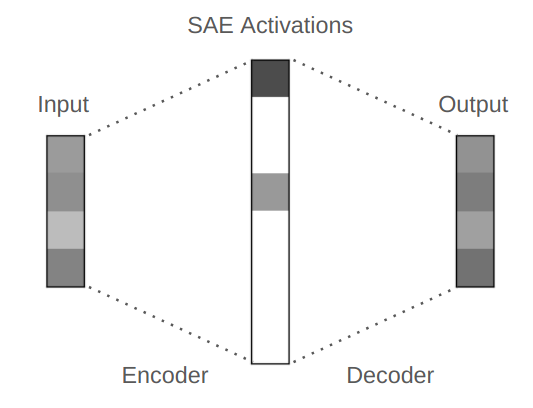
The sparse autoencoder is meant to resolve some of these limitations. In particular, the dimension of the feature space can be equal to or even higher than that of the data space, as illustrated in Figure 6.6. However, the features are required to be highly sparse in the feature space. So if we impose sparsity as a measure of parsimony in addition to rate reduction in the objective (6.1.5), we obtain a new objective for sparse autoencoding:
where the \(\ell ^0\)-“norm” \(\|\spcdot \|_0\) is known to promote sparsity. This is very similar to the sparse rate reduction objective (5.2.4) which we used in the previous Chapter 5 to derive the white-box CRATE architecture.
As a method for learning autoencoding pairs in an end-to-end fashion, sparse autoencoding has been practiced in the past [LRM+12; RPC+06], but nearly all modern autoencoding frameworks are instead based on a different, probabilistic autoencoding framework, which we will study now.
An improved, more modern methodology for autoencoding that still finds significant application to this day is variational autoencoding [KW13a; KW19]. It formulates the representation learning problem in probabilistic terms, as the search for a model \(p(\vx ; \vtheta )\) that maximizes the likelihood of a data sample (or more generally, the population data distribution):
By conditioning we may write \(p(\vx , \vz ;\, \vtheta ) = p(\vz ;\, \vtheta ) p(\vx \mid \vz ;\, \vtheta )\), and
This implies that a probabilistic model for \(\vx \) can be learned with a prior \(p(\vz )\) and a conditional distribution \(p(\vx \mid \vz )\), corresponding more generally to a decoder. Technically, Bayes’ rule then implies that the posterior \(p(\vz \mid \vx )\), necessary for encoding, can be expressed in terms of the prior and the decoder (and samples of \(\vx \)), but this is computationally intractable. Hence, in the VAE framework, we introduce an “approximate posterior” \(q(\vz \mid \vx ;\, \veta )\), corresponding to a separate encoder network, and jointly learn the encoder and decoder through the maximization of a lower bound on the true likelihood, known as the evidence lower bound (ELBO), which is tight when the posterior approximation is tight.
The following instantiation is standard in practice. We use the following Gaussian distributions:
where \(g = (g_1, g_2)\) are deep networks with parameters \(\vtheta \), which correspond to the decoder in the autoencoder. Similarly, for the approximate posterior, we use a Gaussian distribution with parameters given by an encoder MLP \(f = (f_1, f_2)\) with parameters \(\veta \):
This makes probabilistic encoding and decoding simple: we simply map our data \(\vx \) to the mean and variance parameters of a Gaussian distribution for encoding, and vice versa for decoding. After the aforementioned manipulations, the final VAE objective reads:
We can understand this as a regularized autoencoding objective, where there is an interesting additional consistency enforcement in the first term of the ELBO.
At the same time, the reader should note the numerous arbitrary decisions the VAE formalism makes (e.g., the choice and parameterization of the Gaussian distributions). This leads to a complex training objective that remains a challenge to optimize efficiently despite more than ten years of research. Recent representation learning methodologies have made notable improvements to this baseline, and they can even be formulated in the white-box framework we have developed in Chapter 5, as we will soon see.
VAE-Based Latent Diffusion. An important application of VAEs is in the context of latent diffusion models [RBL+22], where a VAE is first trained to learn a more compact and regulated latent representation of high-dimensional data such as images. Then a diffusion model can be trained in the latent space to access the distribution of the representation and hence generate new samples from it, as illustrated in Figure 6.7.
This approach enables efficient generation of high-quality images by leveraging the highly-compressed structure of the learned latent space.6 However, training VAEs can be challenging due to issues such as posterior collapse and balancing the reconstruction and regularization terms in the ELBO. Moreover, the Gaussian posteriors in VAEs are applied per data point and no joint structure is learned across samples, which can severely limit the quality of the learned representations. These challenges have motivated the development of alternative approaches, such as representation autoencoders (RAEs) to be introduced next, which aim to address some of the limitations of VAEs while still providing effective latent representations for generative modeling tasks.
The previous approaches to training autoencoding pairs for representation learning share a common limitation: they do not explicitly organize the representation space \(\vZ \), but only encourage it indirectly (e.g., by enforcing sparsity in the sparse autoencoder or Gaussianity in VAE). As we hinted at the start of the chapter, we have seen previously (in Chapter 4) how to do much better, by learning a representation \(\vZ \) via maximizing the rate reduction \(\Delta R_{\epsilon }(\vZ )\) while ensuring reconstruction consistency. We describe this procedure in more detail in this section, in particular also demonstrating how to efficiently sample in the learned representation space \(\vZ \).
As we have seen at the end of Chapter 4 (Section 4.3), we often can learn a good representation \(\Z \) of the data \(\X \):
based on some end-to-end supervised or self-supervised methods, including the MCR\(^2\) and SimDINO methods introduced in Section 4.3.1 and Section 4.3.2, respectively. As we have also argued, the so-learned representations have better structures than the original data distribution. The representations tend to be a mixture of low-dimensional linear subspaces (or low-rank Gaussians). However, we have not answered the question of how to assess the goodness of the so-learned representations. That is, can we establish from them a reverse decoder:
such that \(\hat \X \) and \(\X \) are close? In light of the preceding examples of classical autoencoding setups, we should expect that an objective of the form (6.1.5) should work—but what sample-wise consistency loss should be used?
Furthermore, those low-dimensional (linear) structures are still embedded in a high-dimensional representation space. Hence, in order to use the so-learned representations, we need to be able to access their distributions too. In Chapter 3, we have learned that denoising is a general approach to identify and hence access such low-dimensional representations. Hence, we can access the distribution of the learned features via a (learned) denoising process from a random noise:
In addition, we have also learned that if the target distribution of \(\Z \) can be modeled (approximately) as a mixture of subspaces or low-rank Gaussians, their optimal denoising operators share a similar structure to those found in Transformers, or in CRATE introduced in Chapter 5.
Thus, altogether, we want to learn an autoencoder for the data \(\X \) whose representation \(\Z \) can be easily accessed. Concretely, we would like to learn an encoder \(f\) and a decoder \(g\) such that:
Figure 6.8 illustrates the above overall processes.
From Chapter 4, we know that the learned representation \(\Z \) by optimizing the (unsupervised) MCR\(^2\) objective satisfies the second requirement and can be viewed to have structures close to a mixture of subspaces or low-rank Gaussians. By incorporating a sample-consistency objective, we can extend the rate reduction objective in Section 4.3.2 to learn a consistent representation:
where \(d(\X , \hat \X )\) is a measure of similarity between the original data \(\X \) and the reconstructed data \(\hat \X = g(\Z )\). In practice, because the objective \(\Delta R_{\epsilon }(\Z )\) alone already promotes low-dimensional structure of \(\Z \), we can pretrain the encoder \(f\) to maximize \(\Delta R_{\epsilon }(\Z )\) first, and then learn the decoder \(g\) to minimize the reconstruction loss \(d(\X , \hat \X )\) while fixing the encoder \(f\). This two-step approach has been demonstrated to be effective, as we will see in Section 8.6.2 of Chapter 8.
Once we have learned such a consistent representation \(\Z \), we can then learn a denoiser to access its distribution, as we have studied in Chapter 3. Concretely, suppose we have a probabilistic model \(p(\z )\) that captures the (marginal) distribution of the learned representations \(\vZ \) and an initial standard Gaussian distribution \(\cN (\Zero , \vI )\). Our goal is to learn a denoiser \(\bar {\z }\) such that it iteratively denoises a sample from the initial distribution to the target distribution of the learned representations. This denoiser can be trained using objectives introduced in Chapter 3 (see also Chapter 7 for conditional denoisers). For instance, take the simple case of flow matching (recall Exercise 3.5 and Section 3.2.2). We can define the denoiser as a time-dependent vector field \(\bar {\z }_{\theta }(t, \z _t)\) parameterized by \(\theta \) that transforms a sample from the initial distribution to the target distribution over time \(t \in [0, 1]\). Here, \(\z _t\) is an interpolation between \(\z _0\) and \(\z _1\) at time \(t\):
where \(\z _0 \sim p(\z )\) is a sample from the learned representation distribution and \(\z _1 \sim \cN (\Zero , \vI )\). The training objective for the denoiser can then be expressed as:
It is worth noting the difference between learning a denoiser for the representations learned via VAE and those learned via methods like MCR\(^2\) or SimDINO. As discussed in Section 6.1.4, the VAE representations are enforced to approximate a Gaussian posterior per sample and no joint distribution of the latent space is modeled, making the representation space less structured and the denoising process potentially more challenging. In contrast, representations learned through MCR\(^2\) or SimDINO tend to have more pronounced linear and low-dimensional structures, such as mixtures of subspaces or low-rank Gaussians (as demonstrated in Section 4.3.2), which can facilitate the denoising process. This structural property can lead to more efficient and effective denoising models, as they can better exploit the underlying geometry of the representation space.
Once we have trained the denoiser, we can use it to generate new samples from the learned representation distribution via a diffusion process, as we have shown in Chapter 3. This completes the learning of a representation autoencoder (RAE) with an accessible representation distribution. In Chapter 8 (specifically Section 8.6.2), we will see a specific implementation of RAE and its applications in image generation.
In earlier chapters, we have studied methods that would allow us to learn a low-dimensional distribution via (lossy) compression. As we have mentioned in Chapter 1 and demonstrated in the previous chapters, the progress made in machine intelligence largely relies on finding computationally feasible and efficient solutions to realize the desired compression, not only computable or tractable in theory, but also scalable in practice:
It is even fair to say that the tremendous advancement in machine intelligence made in the past decade or so is largely attributed to the development of scalable models and methods, say by training deep networks via back propagation. Large models with billions of parameters trained with trillions of data points on tens of thousands of powerful GPUs have demonstrated super-human capabilities in memorizing existing knowledge. This has led many to believe that the “intelligence” of such models will continue to improve as their scale continues to go up.
While we celebrate the engineering marvels of such large man-made machine learning systems, we also must admit that, compared to intelligence in nature, this approach to improving machine intelligence is unnecessarily resource-demanding. Natural intelligent beings, including animals and humans, simply cannot afford such a brute-force solution for learning because they must operate with a very limited budget in energy, space, and time, subject to many strict physical constraints.
First, there is strong scientific evidence that our brain does not conduct global end-to-end back propagation to improve or correct its predictions. Instead, it has long been known in neuroscience that our brain corrects errors with local closed-loop feedback, such as predictive coding. This was the scientific basis that inspired Norbert Wiener to develop the theory of feedback control and the Cybernetics program back in the 1940s.
Second, we saw in the previous sections that in order to learn a consistent representation, one needs to learn a bidirectional autoencoding:
It requires enforcing the observed input data \(\X \) and the decoded \(\hat \X \) to be close by some measure of similarity \(d(\X , \hat \X )\). However, when the data \(\X \) is high-dimensional (e.g., images), naive distance measures such as the \(\ell ^2\) norm in ambient space are largely uninformative: two images that differ by a small geometric transformation may be far apart in pixel distance yet perceptually identical. Hence, an outstanding question is: how can we enforce similarity between \(\X \) and \(\hat \X \) without a meaningful distance in the ambient data space? As we will see in this chapter, the answer lies in closed-loop feedback in a learned feature space, together with the low-dimensionality of the data distribution.
As we know from the previous chapter, in order to ensure that a representation is consistent, we need to compare the generated \(\hat \X \sim p(\hat \x )\) and the original \(\X \sim p(\x )\), at least in distribution. Even when we do have access to \(\X \) and \(\hat \X \), technically, computing and minimizing the distance between two distributions can be problematic, especially when the support of the distributions is low-dimensional. The KL-divergence introduced in Chapter 3 is not even well-defined between two distributions that do not have overlapping supports.
As an early attempt to alleviate the above difficulty in computing and minimizing the distance between two (low-dimensional) distributions, people had suggested learning the generator/decoder \(g\) via discriminative approaches [Tu07]. This line of thought has led to the idea of Generative Adversarial Nets (GAN) [GPM+14b]. It introduces a discriminator \(d\), usually modeled by a deep network, to discern differences between the generated samples \(\hat \X \) and the real ones \(\X \):
It is suggested that we may attempt to align the distributions between \(\hat \x \) and \(\x \) via a Stackelberg game—a sequential game in which one player (the leader) commits to a strategy first and the other (the follower) responds optimally (see Section A.3 for a detailed treatment)—between the generator \(g\) and the discriminator \(d\):
That is, the discriminator \(d\) is trying to minimize the cross entropy between the true samples \(\X \) and the generated ones \(\hat \X \) while the generator \(g\) is trying to do the opposite.
One may show that finding an equilibrium for the above Stackelberg game is equivalent to minimizing the Jensen-Shannon divergence:
Note that, compared to the KL-divergence, the JS-divergence is well-defined even if the supports of the two distributions are non-overlapping. However, JS-divergence does not have a closed-form expression even between two Gaussians, whereas KL-divergence does. In addition, since the data distributions are low-dimensional, the JS-divergence can be highly ill-conditioned to optimize.7 This may explain why many additional heuristics are typically used in many subsequent variants of GAN.
So, instead, it has also been suggested to replace JS-divergence with the earth mover (EM) distance or the Wasserstein distance.8 However, both the JS-divergence and Wasserstein distance can only be approximately computed between two general distributions.9 Furthermore, neither the JS-divergence nor the Wasserstein distance has closed-form formulae, even for Gaussian distributions.10
If it is difficult to compare distributions of the data \(\X \) and \(\hat \X \), it may be possible to compare the learned feature \(\Z \) with its image \(\hat \Z \) under the encoder \(f\):
This leads to the notion of self-consistent representation.
Definition 6.2 (Self-Consistent Representation). Given data \(\vX \), we call a self-consistent representation a pair of functions \((f \colon \cX \to \cZ , g \colon \cZ \to \cX )\), such that the features \(\vZ = f(\vX )\) are compact and structured, and the autoencoding features \(\hat {\vZ } \doteq f \circ g(\vZ )\) are close to \(\vZ \).
How do we try to ensure a learned representation is self-consistent? As usual, let us assume \(\X = \cup _{k=1}^K \X _k\) with each subset of samples \(\X _k\) belonging to a low-dimensional submanifold: \(\X _k \subset \mathcal {M}_k, k = 1,\ldots , K\). Following the notation in Chapter 3, we use a matrix \(\bm \Pi _k(i,i) = 1\) to denote the membership of sample \(i\) belonging to class \(k\) and \(\bm \Pi _k(i,j) = 0\) otherwise. One seeks a continuous mapping \(f(\cdot ,\bm \theta ): \x \mapsto \z \) from \(\X \) to an optimal representation \(\Z = [\z _1, \ldots , \z _N] \subset \mathbb {R}^{d \times N}\):
which maximizes the following coding rate-reduction (MCR\(^2\)) objective:
where \(\alpha = {d}/({N\epsilon ^2})\), \(\alpha _k = d/({\mathrm {tr}(\bm {\Pi }_k)\epsilon ^2})\), \(\gamma _k = {\mathrm {tr}(\bm {\Pi }_{k})}/{N}\) for each \(k = 1,\dots , K\).
One issue with learning such a one-sided mapping (6.2.7) via maximizing the above objective (6.2.8) is that it tends to expand the dimension of the learned subspace for features in each class11, as we have seen in Section 4.2 of Chapter 4. To verify whether the learned features are consistent, meaning neither over-estimating nor under-estimating the intrinsic data structure, we may consider learning a decoder \(g(\cdot ,\eta ): \z \mapsto \x \) from the representation \(\Z = f(\X ,\bm \theta )\) back to the data space \(\x \): \(\hat \X = g(\Z , \bm \eta )\):
and check how close \(\X \) and \(\hat \X \) are. This forms an autoencoding which is what we have studied extensively earlier in this chapter.
Measuring distance in the feature space. However, as we have discussed above, if we do not have the option to compute the distance between \(\X \) and \(\hat \X \), we are left with the option of comparing their corresponding features \(\Z \) and \(\hat \Z = f(\hat \X , \bm \theta )\). Notice that under the MCR\(^2\) objective, the distributions of the resulting \(\Z \) or \(\hat \Z \) tend to be piecewise linear so their distance can be computed more easily. More precisely, since the features of each class, \(\Z _k\) and \(\hat {\Z }_k\), are close to being a low-dimensional subspace/Gaussian, their “distance” can be measured by the rate reduction, with (6.2.8) restricted to two sets of equal size:
The overall distance between \(\Z \) and \(\hat \Z \) is given by:
If we are interested in discerning any differences in the distributions of the original data \(\X \) and their decoded \(\hat \X \), we may view the feature encoder \(f(\cdot , \bm \theta )\) as a “discriminator” to magnify any difference between all pairs of \(\X _k\) and \(\hat \X _k\), by simply maximizing the distance \(d(\Z , \hat \Z )\):
That is, a “distance” between \(\X \) and \(\hat \X \) can be measured as the maximally achievable rate reduction between all pairs of classes in these two sets. In a way, this measures how well or badly the decoded \(\hat \X \) aligns with the original data \(\X \)—hence measuring the goodness of “injectivity” of the encoder \(f\). Notice that such a discriminative measure is consistent with the idea of GAN (6.2.3) that tries to separate \(\X \) and \(\hat \X \) into two classes, measured by the cross-entropy.
Nevertheless, here the discriminative encoder \(f\) naturally generalizes to cases when the data distributions are multi-class and multi-modal, and the discriminativeness is measured with a more refined measure—the rate reduction—instead of the typical two-class loss (e.g., cross entropy) used in GANs. That is, we may view the encoder \(f\) as a generalized discriminator that replaces the binary classifier \(d\) in (6.2.3):
The overall pipeline can be illustrated by the following “closed-loop” diagram:
where the overall model has parameters: \(\bm \Theta = \{\bm \theta , \bm \eta \}\). Figure 6.9 shows the overall process.
Encoder and decoder as a two-player game. Obviously, to ensure the learned autoencoding is self-consistent, the main goal of the decoder \(g(\cdot , \bm \eta )\) is to minimize the distance between \(\Z \) and \(\hat \Z \). That is, to learn \(g\), we want to minimize the distance \(d(\Z , \hat \Z )\):
where \(\Z _k = f(\X _k,\bm \theta )\) and \(\hat \Z _k = f(\hat {\X }_k,\bm \theta )\).
Example 6.1. One may wonder why we need the mapping \(f(\cdot , \bm \theta )\) to function as a discriminator between \(\X \) and \(\hat \X \) by maximizing \(\max _{\bm \theta } \Delta R_\epsilon \big (f(\X ,\bm \theta ), f(\hat \X , \bm \theta )\big )\). Figure 6.10 gives a simple illustration: there might be many decoders \(g\) such that \(f\circ g\) is an identity (Id) mapping. \(f\circ g(\z ) = \z \) for all \(\z \) in the subspace \(S_{\z }\) in the feature space. However, \(g\circ f\) is not necessarily an autoencoding map for \(\x \) in the original distribution \(S_{\x }\) (here drawn as a subspace for simplicity). That is, \(g\circ f(S_{\x }) \not \subset S_{\x }\), let alone \(g\circ f(S_{\x }) = S_{\x }\) or \(g\circ f(\x ) = \x \). One should expect that, without careful control of the image of \(g\), this would be the case with high probability, especially when the support of the distribution of \(\x \) is extremely low-dimensional in the original high-dimensional data space. \(\blacksquare \)
Comparing the contractive and contrastive nature of (6.2.15) and (6.2.12) on the same distance measure, we see the roles of the encoder \(f(\cdot , \bm \theta )\) and the decoder \(g(\cdot , \bm \eta )\) naturally as “a two-player game”: while the encoder \(f\) tries to magnify the difference between the original data and their transcribed data, the decoder \(g\) aims to minimize the difference. Now for convenience, let us define the “closed-loop encoding” function:
Ideally, we want this function to be very close to \(f(\x , \bm \theta )\) or at least the distributions of their images should be close. With this notation, combining (6.2.15) and (6.2.12), a closed-loop notion of “distance” between \(\X \) and \(\hat \X \) can be computed as an equilibrium point to the following Stackelberg game (cf. Section A.3) for the same utility in terms of rate reduction:
Notice that this only measures the difference between (features of) the original data and its transcribed version. It does not measure how good the representation \(\Z \) (or \(\hat \Z \)) is for the multiple classes within \(\X \) (or \(\hat \X \)). To this end, we may combine the above distance with the original MCR\(^2\)-type objectives (6.2.8): namely, the rate reduction \(\Delta R_\epsilon (\Z )\) and \(\Delta R_\epsilon (\hat \Z )\) for the learned LDR \(\Z \) for \(\X \) and \(\hat \Z \) for the decoded \(\hat \X \). Notice that although the encoder \(f\) tries to maximize the multi-class rate reduction of the features \(\Z \) of the data \(\X \), the decoder \(g\) should minimize the rate reduction of the multi-class features \(\hat \Z \) of the decoded \(\hat \X \). That is, the decoder \(g\) tries to use a minimal coding rate needed to achieve a good decoding quality.
Hence, the overall “multi-class” Stackelberg game for learning the closed-loop transcription, named CTRL-Multi, is
subject to certain constraints (upper or lower bounds) on the first term and the second term.
Notice that, without the terms associated with the generative part \(h\) or with all such terms fixed as constant, the above objective is precisely the original MCR\(^2\) objective introduced in Chapter 4. In an unsupervised setting, if we view each sample (and its augmentations) as its own class, the above formulation remains exactly the same. The number of classes \(K\) is simply the number of independent samples. In addition, notice that the above game’s objective function depends only on (features of) the data \(\X \), hence one can learn the encoder and decoder (parameters) without the need for sampling or matching any additional distribution (as typically needed in GANs or VAEs).
As a special case, if \(\X \) only has one class, the Stackelberg game reduces to a special “two-class” or “binary” form,12 named CTRL-Binary,
between \(\X \) and the decoded \(\hat \X \) by viewing \(\X \) and \(\hat \X \) as two classes \(\{\bm 0, \bm 1\}\). Notice that this binary case resembles the formulation of the original GAN (6.2.3). Instead of using cross entropy, our formulation adopts a more refined rate-reduction measure, which has been shown to promote diversity in the learned representation in Chapter 3.
Sometimes, even when \(\X \) contains multiple classes/modes, one could still view all classes together as one class. Then, the above binary objective is to align the union distribution of all classes with their decoded \(\hat \X \). This is typically a simpler task to achieve than the multi-class one (6.2.20), since it does not require learning of a more refined multi-class CTRL for the data, as we will later see in experiments. Notice that one good characteristic of the above formulation is that all quantities in the objectives are measured in terms of rate reduction for the learned features (assuming features eventually become subspace Gaussians).
One may notice that the above learning framework draws inspiration from closed-loop error correction widely practiced in feedback control systems. The closed-loop mechanism is used to form an overall feedback system between the two encoding and decoding networks for correcting any “error” in the distributions between the data \(\x \) and the decoded \(\hat \x \). Using terminology from control theory, one may view the encoding network \(f\) as a “sensor” for error feedback while the decoding network \(g\) as a “controller” for error correction. However, notice that here the “target” for control is not a scalar nor a finite dimensional vector, but a continuous distribution—in order for the distribution of \(\hat \x \) to match that of the data \(\x \). This is in general a control problem in an infinite dimensional space. The space of possible diffeomorphisms of submanifolds that \(f\) tries to model is infinite-dimensional [Lee02]. Ideally, we hope when the sensor \(f\) and the controller \(g\) are optimal, the distribution of \(\x \) becomes a “fixed point” for the closed loop while the distribution of \(\z \) reaches a compact linear discriminative representation. Hence, the minimax programs (6.2.20) and (6.2.21) can also be interpreted as games between an error-feedback sensor and an error-reducing controller.
The remaining question is whether the above framework can indeed learn a good (autoencoding) representation of a given dataset? Before we give some formal theoretical justification (in the next subsection), we present some empirical results.
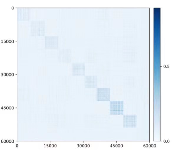
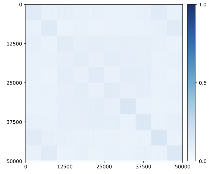
Visualizing correlation of features \(\Z \) and decoded features \(\hat \Z \). We visualize the cosine similarity between \(\Z \) and \(\hat {\Z }\) learned from the multi-class objective (6.2.20) on MNIST, CIFAR-10 and ImageNet (10 classes), which indicates how close \(\hat {\z } = f\circ g(\z )\) is from \(\z \). Results in Figure 6.11 show that \(\Z \) and \(\hat {\Z }\) are aligned very well within each class. The block-diagonal patterns for MNIST are sharper than those for CIFAR-10 and ImageNet, as images in CIFAR-10 and ImageNet have more diverse visual appearances.
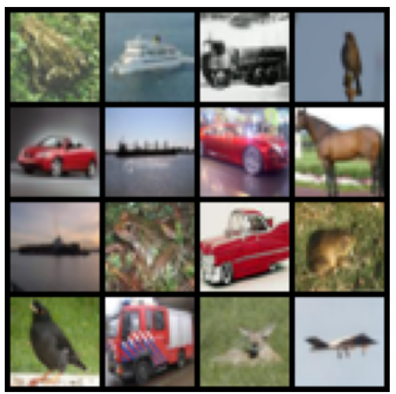
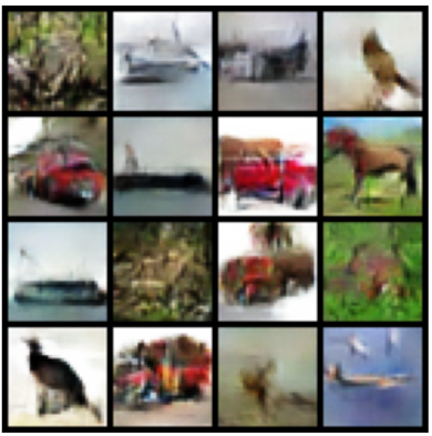
Visualizing autoencoding of the data \(\X \) and the decoded \(\hat \X \). We compare some representative \(\X \) and \(\hat {\X }\) on MNIST, CIFAR-10 and ImageNet (10 classes) to verify how close \(\hat \x = g\circ f(\x )\) is to \(\x \). The results are shown in Figure 6.12, and visualizations are created from training samples. Visually, the autoencoded \(\hat \x \) faithfully captures major visual features from its respective training sample \(\x \), especially the pose, shape, and layout. For the simpler dataset such as MNIST, autoencoded images are almost identical to the original.
In the above, we have argued that it is possible to formulate the problem of learning a data distribution as a closed-loop autoencoding problem. We also saw empirically that such a scheme seems to work. The remaining question is when and why such a scheme should work. It is difficult to answer this question for the most general cases with arbitrary data distributions. Nevertheless, as usual, let us see if we can arrive at a rigorous justification for the ideal case when the data distribution is a mixture of low-dimensional subspaces or low-rank Gaussians. A clear characterization and understanding of this important special case would shed light on the more general cases.13
To this end, let us first suppose that \(\vX \) is distributed according to a mixture of low-dimensional Gaussians, and the label (i.e., subspace assignment) for \(\vX \) is given by \(\vy \). Then, let us set up a minimax optimization problem to learn the data distribution, say through learning an encoding of \(\vX \) into representations \(\vZ \) which are supported on a mixture of orthogonal subspaces, and a decoding of \(\vZ \) back into \(\vX \). Then, the representation we want to achieve is maximized by the earlier-discussed version of the information gain, i.e., \( \Delta R_{\epsilon }(\vZ ) = R_{\epsilon }(\vZ ) - \sum _{k=1}^K R_{\epsilon }(\vZ _{k}) \), which enforces that the representation \(\vZ _{k}\) of each class \(k\) spans a subspace which is orthogonal to the supporting subspaces of other classes. The way to measure the consistency of the decoding is, as before, given by \(\sum _{k = 1}^{K}\Delta R_\epsilon (\vZ _{k}, \hat {\vZ }_{k})\), which enforces that the representation \(\vZ _{k}\) and its autoencoding \(\hat {\vZ }_{k}\) for each class \(k\) span the same subspace. Thus, we can set up a simplified Stackelberg game:
Notice that this is a simpler setup than what is used in practice—there is no \(\Delta R_\epsilon (\hat {\vZ })\) term, for instance, and we work in the supervised setting with class labels (although the techniques used to prove the following result are easy to extend to unsupervised formulations). Also, the consistency of the representations is only measured in a distribution-wise sense via \(\Delta R_\epsilon \) (though this may be substituted with a sample-wise distance metric such as the \(\ell _{2}\) norm if desired, and equivalent conclusions may be drawn, mutatis mutandis).
Under mild conditions, in order to realize the desired encoder and decoder which realize \(\vZ \) from a data source \(\vX \) that is already distributed according to a mixture of correlated low-dimensional Gaussians, we only require a linear encoder and decoder to disentangle and whiten the Gaussians. We then study this setting in the case where \(\bm \theta \) and \(\bm \eta \) parameterize matrices whose operator norm is constrained.
We want to understand what kinds of optima are learned in this setting. One suitable solution concept for this kind of game, where the decoder’s optimal solution is defined solely with respect to the encoder (and not, in particular, with respect to some other intrinsic property of the decoder), is a Stackelberg equilibrium where the decoder follows the encoder. Namely, at such an equilibrium, the decoder should optimize its objective; meanwhile the encoder should optimize its objective, given that whatever it picks, the decoder will pick an optimal response (which may affect the encoder objective). In game-theoretic terms, it is like the decoder goes second: it chooses its weights after the encoder, and both the encoder and decoder attempt to optimize their objective in light of this. It is computationally tractable to learn sequential equilibria via gradient methods via alternating optimization, where each side uses different learning rates. Detailed exposition of sequential equilibria is beyond the scope of this book and we provide more technical details in Section A.3. In this setting, we have the following result:
Theorem 6.1 ([PPC+23], Abridged). Suppose that \(\vX \) is distributed on a mixture of subspaces. Under certain realistic yet technical conditions, it holds that all sequential equilibria of (6.2.22) obey:
This notion of self-consistency is the most one can expect if there are only geometric assumptions on the data, i.e., there are no statistical assumptions. If we assume that the columns of \(\vX \) are drawn from a low-rank Gaussian mixture model, then analogous versions of this theorem certify that \(\vZ _{k}\) are also low-rank Gaussians whose covariance is isotropic, for instance. Essentially, this result validates, via the simple case of Gaussian mixtures on subspaces, that minimax games to optimize the information gain and self-consistency may achieve optimal solutions.
As we have seen, deep neural networks have demonstrated a great ability to learn representations for hundreds or even thousands of classes of objects, in both discriminative and generative contexts. However, networks typically must be trained offline, with uniformly sampled data from all classes simultaneously. It has been known that when an (open-loop) network is updated to learn new classes without data from the old ones, previously learned knowledge will fall victim to the problem of catastrophic forgetting [MC89]. This is known in neuroscience as the stability-plasticity dilemma: the challenge of ensuring that a neural system can learn from a new environment while retaining essential knowledge from previous ones [Gro87].
In contrast, natural neural systems (e.g., animal brains) do not seem to suffer from such catastrophic forgetting at all. They are capable of developing new memory of new objects while retaining memory of previously learned objects. This ability, for either natural or artificial neural systems, is often referred to as incremental learning, continual learning, sequential learning, or lifelong learning [AR20].
While many recent works have highlighted how artificial neural systems can be trained in more flexible ways, the strongest existing efforts toward answering the stability-plasticity dilemma for artificial neural networks typically require either storing raw exemplars [CRE+19; RKS+17] or providing external mechanisms [KPR+17]. Raw exemplars, particularly in the case of high-dimensional inputs like images, are costly and difficult to scale, while external mechanisms—which typically include secondary networks and representation spaces for generative replay, incremental allocation of network resources, network duplication, or explicit isolation of used and unused parts of the network—require heuristics and incur hidden costs.
Here we are interested in an incremental learning setting that is similar to nature. It counters these existing practices with two key qualities.
The incoherent linear structures for features of different classes closely resemble how objects are encoded in different areas of the inferotemporal cortex of animal brains [BSM+20; CT17]. The closed-loop transcription \(\X \rightarrow \Z \rightarrow \hat {\X } \rightarrow \hat {\Z }\) also resembles popularly hypothesized mechanisms for memory formation [JT20; VST+20]. This leads to a question: since memory in the brain is formed in an incremental fashion, can the above closed-loop transcription framework also support incremental learning?
LDR memory sampling and replay. The simple linear structures of LDR make it uniquely suited for incremental learning: the distribution of features \(\Z _j\) of each previously learned class can be explicitly and concisely represented by a principal subspace \(\mathcal {S}_j\) in the feature space. To preserve the memory of an old class \(j\), we only need to preserve the subspace while learning new classes. To this end, we simply sample \(m\) representative prototype features on the subspace along its top \(r\) principal components, and denote these features as \(\Z _{j,old}\). Because of the simple linear structures of LDR, we can sample from \(\Z _{j,old}\) by calculating the mean and covariance of \(\Z _{j,old}\) after learning class \(j\). The storage required is extremely small, since we only need to store means and covariances, which are sampled from as needed. Suppose a total of \(t\) old classes have been learned so far. If prototype features, denoted \(\Z _{old} \doteq [\Z _{1,old},\ldots , \Z _{t,old}]\), for all of these classes can be preserved when learning new classes, the subspaces \(\{\mathcal {S}_j\}_{j=1}^t\) representing past memory will be preserved as well. Details about sampling and calculating mean and covariance can be found in the work of [TDW+23].
Incremental learning LDR with an old-memory constraint. Notice that, with the learned autoencoding (6.2.9), one can replay and use the images, say \(\hat \X _{old} = g(\Z _{old}, \bm \eta )\), associated with the memory features to avoid forgetting while learning new classes. This is typically how generative models have been used for prior incremental learning methods. However, with the closed-loop framework, explicitly replaying images from the features is not necessary. Past memory can be effectively preserved through optimization exclusively on the features themselves.
Consider the task of incrementally learning a new class of objects.14 We denote a corresponding new sample set as \(\X _{new}\). The features of \(\X _{new}\) are denoted as \(\Z _{new}(\bm \theta ) = f(\X _{new}, \bm \theta )\). We concatenate them together with the prototype features of the old classes \(\Z _{old}\) and form \(\Z = [\Z _{new}(\bm \theta ), \Z _{old}]\). We denote the replayed images from all features as \(\hat {\X } = [{\hat {\X }_{new}(\bm \theta ,\bm \eta )}, {\hat {\X }_{old}(\bm \eta )}]\) although we do not actually need to compute or use them explicitly. We only need features of replayed images, denoted \(\hat {\Z } = f(\hat {\X }, \bm \theta ) = [{\hat {\Z }_{new}(\bm \theta ,\bm \eta )}, {\hat {\Z }_{old}(\bm \theta ,\bm \eta )}]\).
Mirroring the motivation for the multi-class CTRL objective (6.2.20), we would like the features of the new class \(\Z _{new}\) to be incoherent to all of the old ones \(\Z _{old}\). As \(\Z _{new}\) is the only new class whose features need to be learned, the objective (6.2.20) reduces to the case where \(K=1\):
However, when we update the network parameters \((\bm \theta ,\bm \eta )\) to optimize the features for the new class, the updated mappings \(f\) and \(g\) will change features of the old classes too. Hence, to minimize the distortion of the old class representations, we can try to enforce \(\mbox {Cov}(\Z _{j,old}) = \mbox {Cov}(\hat {\Z }_{j,old})\). In other words, while learning new classes, we enforce that the memory of old classes remains “self-consistent” through the transcription loop:
Mathematically, this is equivalent to setting
Hence, the above minimax program (6.3.1) is revised as a constrained minimax game, which we refer to as incremental closed-loop transcription (i-CTRL). The objective of this game is identical to the standard multi-class CTRL objective (6.2.20), but includes just one additional constraint:
In practice, the constrained minimax program can be solved by alternating minimization and maximization between the encoder \(f(\cdot , \bm \theta )\) and decoder \(g(\cdot , \bm \eta )\) as follows:
where the constraint \(\Delta R_\epsilon (\Z _{old},\hat {\Z }_{old}) = 0\) in (6.3.3) has been converted (and relaxed) to a Lagrangian term with a corresponding coefficient \(\gamma \) and sign. We additionally introduce another coefficient \(\lambda \) for weighting the rate reduction term associated with the new data.
Jointly optimal memory via incremental reviewing. As we will see, the above constrained minimax program can already achieve state-of-the-art performance for incremental learning. Nevertheless, developing an optimal memory for all classes cannot rely on graceful forgetting alone. Even for humans, if an object class is learned only once, we should expect the learned memory to fade as we continue to learn new ones, unless the memory can be consolidated by reviewing old object classes.
To emulate this phase of memory forming, after incrementally learning a whole dataset, we may go back to review all classes again, one class at a time. We refer to going through all classes once as one reviewing “cycle”.15 If needed, multiple reviewing cycles can be conducted. It is quite expected that reviewing can improve the learned (LDR) memory. But somewhat surprisingly, the closed-loop framework allows us to review even in a “class-unsupervised” manner: when reviewing data of an old class, say \(\X _j\), the system does not need the class label and can simply treat \(\X _j\) as a new class \(\X _{new}\). That is, the system optimizes the same constrained mini-max program (6.3.3) without any modification; after the system is optimized, one can identify the newly learned subspace spanned by \(\Z _{new}\), and use it to replace or merge with the old subspace \(\mathcal {S}_j\). As our experiments show, such a class-unsupervised incremental review process can gradually improve both discriminative and generative performance of the LDR memory, eventually converging to that of a jointly learned memory.
Experimental verification. We show some experimental results on the following datasets: MNIST [LBB+98b] and CIFAR-10 [KNH14]. All experiments are conducted for the more challenging class-IL setting. For both MNIST and CIFAR-10, the 10 classes are split into 5 tasks with 2 classes each or 10 tasks with 1 class each. For the encoder \(f\) and decoder \(g\), we adopt a very simple network architecture modified from DCGAN [RMC16], which is merely a four-layer convolutional network. Here we only show some qualitative visual results; more experiments and detailed analysis can be found in the work [TDW+23].
Visualizing auto-encoding properties. We begin by qualitatively visualizing some representative images \(\X \) and the corresponding replayed \(\hat {\X }\) on MNIST and CIFAR-10. The model is learned incrementally with the datasets split into 5 tasks. Results are shown in Figure 6.14, where we observe that the reconstructed \(\hat {\X }\) preserves the main visual characteristics of \(\X \) including shapes and textures. For a simpler dataset like MNIST, the replayed \(\hat {\X }\) are almost identical to the input \(\X \)! This is rather remarkable given: (1) our method does not explicitly enforce \(\hat {\x } \approx \x \) for individual samples as most autoencoding methods do, and (2) after having incrementally learned all classes, the generator has not forgotten how to generate digits learned earlier, such as 0, 1, 2. For a more complex dataset like CIFAR-10, we also demonstrate good visual quality, faithfully capturing the essence of each image.
Principal subspaces of the learned features. Most generative memory-based methods utilize autoencoders, VAEs, or GANs for replay purposes. The structure or distribution of the learned features \(\Z _j\) for each class is unclear in the feature space. The features \(\Z _j\) of the LDR memory, on the other hand, have a clear linear structure. Figure 6.15 visualizes correlations among all learned features \(|\Z ^\top \Z |\), in which we observe clear block-diagonal patterns for both datasets.16 This indicates that the features for different classes \(\Z _j\) indeed lie on subspaces that are incoherent from one another. Hence, features of each class can be well modeled as a principal subspace in the feature space.
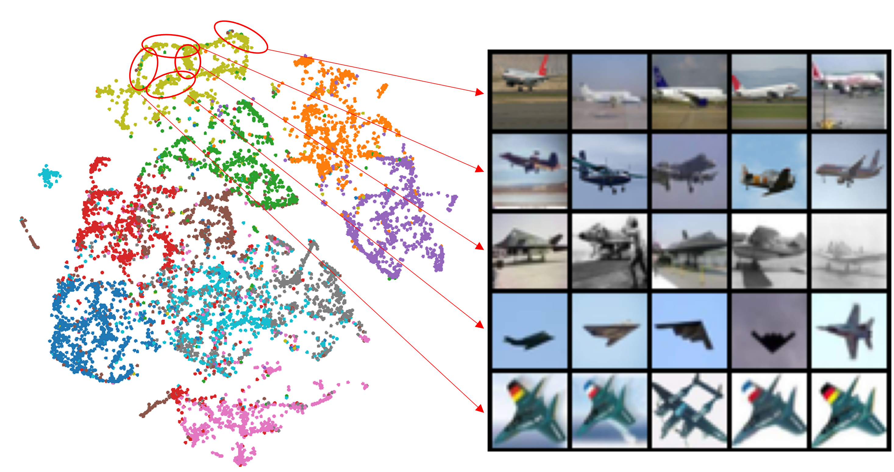
Replay images of samples from principal components. Since features of each class can be modeled as a principal subspace, we further visualize the individual principal components within each of those subspaces. Figure 6.16 shows the images replayed from sampled features along the top-4 principal components for different classes, on MNIST and CIFAR-10 respectively. Each row represents samples along one principal component, and they clearly show similar visual characteristics but are distinctively different from those in other rows. We see that the model remembers different poses of ‘4’ after having learned all remaining classes. For CIFAR-10, the incrementally learned memory remembers representative poses and shapes of horses and ships.
Effectiveness of incremental reviewing. We verify how the incrementally learned LDR memory can be further consolidated with an unsupervised incremental reviewing phase described before. Experiments are conducted on CIFAR-10, with 10 steps. Figure 6.17 left shows replayed images of the first class ‘airplane’ at the end of incremental learning of all ten classes, sampled along the top-3 principal components – every two rows (16 images) are along one principal direction. Their visual quality remains very decent—we observe almost no forgetting. The right figure shows replayed images after reviewing the first class once. We notice a significant improvement in visual quality after reviewing, and principal components of the features in the subspace start to correspond to distinctively different visual attributes within the same class.
As we know, the closed-loop CTRL formulation can already learn a decent autoencoding, even without class information, with the CTRL-Binary program:
However, note that (6.3.6) is practically limited because it only aligns the dataset \(\X \) and the regenerated \(\hat \X \) at the distribution level. There is no guarantee that each sample \(\x \) would be close to the decoded \(\hat \x = g(f(\x ))\).
Sample-wise constraints for unsupervised transcription. To improve discriminative and generative properties of representations learned in the unsupervised setting, we propose two additional mechanisms for the above CTRL-Binary maximin game (6.3.6). For simplicity and uniformity, here these will be formulated as equality constraints over rate reduction measures, but in practice they can be enforced softly during optimization.
Sample-wise self-consistency via closed-loop transcription. First, to address the issue that CTRL-Binary does not learn a sample-wise consistent autoencoding, we need to promote \(\hat \x \) to be close to \(\x \) for each sample. In the CTRL framework, this can be achieved by enforcing their corresponding features \(\z =f(\x )\) and \(\hat \z = f(\hat \x )\) to be close. To promote sample-wise self-consistency, where \(\hat {\x } = g(f(\x ))\) is close to \(\x \), we want the distance between \(\z \) and \(\hat {\z }\) to be zero or small, for all \(N\) samples. This distance can be measured by the rate reduction:
Note that this again avoids measuring differences in the image space.
Self-supervision via compressing augmented samples. Since we do not know any class label information between samples in the unsupervised setting, the best we can do is to view every sample and its augmentations (say via translation, rotation, occlusion, etc.) as one “class”—a basic idea behind almost all self-supervised learning methods. In the rate reduction framework, it is natural to compress the features of each sample and its augmentations. In this work, we adopt the standard transformations in SimCLR [CKN+20] and denote such a transformation as \(\tau \). We denote each augmented sample \(\x _a = \tau (\x )\), and its corresponding feature as \(\z _a = f(\x _a, \bm \theta )\). For discriminative purposes, we hope the classifier is invariant to such transformations. Hence it is natural to enforce that the features \(\z _a\) of all augmentations are the same as those \(\z \) of the original sample \(\x \). This is equivalent to requiring the distance between \(\z \) and \(\z _a\), measured in terms of rate reduction again, to be zero (or small) for all \(N\) samples:
Unsupervised representation learning via closed-loop transcription. So far, we know the CTRL-Binary objective \(\Delta R_\epsilon (\Z , \hat {\Z })\) in (6.3.6) helps align the distributions while sample-wise self-consistency (6.3.7) and sample-wise augmentation (6.3.8) help align and compress features associated with each sample. Besides consistency, we also want learned representations to be maximally discriminative for different samples (here viewed as different “classes”). Notice that the rate distortion term \(R_\epsilon (\Z )\) measures the coding rate (hence volume) of all features.
Unsupervised CTRL. Putting these elements together, we propose to learn a representation via the following constrained maximin program, which we refer to as unsupervised CTRL (u-CTRL):
Figure 6.18 illustrates the overall architecture of the closed-loop system associated with this program.
In practice, the above program can be optimized by alternating maximization and minimization between the encoder \(f(\cdot ,\bm \theta )\) and the decoder \(g(\cdot ,\bm \eta )\). We adopt the following optimization strategy that works well in practice, which is used for all subsequent experiments on real image datasets:
where the constraints \(\sum _{i\in N} \Delta R_\epsilon (\z ^i, \hat {\z }^i) = 0\) and \(\sum _{i\in N} \Delta R_\epsilon (\z ^i, \z _{a}^i) = 0\) in (6.3.9) have been converted (and relaxed) to Lagrangian terms with corresponding coefficients \(\lambda _{1}\) and \(\lambda _{2}\).17
The above representation is learned without class information. In order to facilitate discriminative or generative tasks, it must be highly structured. It has been verified experimentally that this is indeed the case and u-CTRL demonstrates significant advantages over other incremental or unsupervised learning methods [TDC+24]. We here only illustrate some qualitative results with the experiment on the CIFAR-10 dataset [KNH14], with standard augmentations for self-supervised learning [CKN+20]. One may refer to [TDC+24] for experiments on more and larger datasets and their quantitative evaluations.
As one can see from the experiments, specific and unique structure indeed emerges naturally in the representations learned using u-CTRL: globally, features of images in the same class tend to be clustered well together and separated from other classes, as shown in Figure 6.19; locally, features of individual classes cluster into tight, well-separated groups, as shown in Figure 6.20.
Unsupervised conditional image generation via rate reduction. The highly-structured feature distribution also suggests that the learned representation can be very useful for generative purposes. For example, we can organize the sample features into meaningful clusters, and model them with low-dimensional (Gaussian) distributions or subspaces. By sampling from these compact models, we can conditionally regenerate meaningful samples from computed clusters. This is known as unsupervised conditional image generation [HKJ+21].
To cluster features, we exploit the fact that the rate reduction framework (4.2.15) is inspired by unsupervised clustering via compression [MDH+07b], which provides a principled way to find the membership \(\bm \Pi \). Concretely, we maximize the same rate reduction objective (4.2.15) over \(\bm \Pi \), but fix the learned representation \(\Z \) instead. We simply view the membership \(\bm \Pi \) as a nonlinear function of the features \(\Z \), say \(h_{\bm \pi }(\cdot ,\xi ):\Z \mapsto \bm \Pi \) with parameters \(\xi \). In practice, we model this function with a simple neural network, such as an MLP head right after the output feature \(\z \). To estimate a “pseudo” membership \(\hat {\bm \Pi }\) of the samples, we solve the following optimization problem over \(\bm \Pi \):
In Figure 6.21, we visualize images generated from the ten unsupervised clusters from (6.3.12). Each block represents one cluster and each row represents one principal component for each cluster. Despite learning and training without labels, the model not only organizes samples into correct clusters, but is also able to preserve statistical diversities within each cluster/class. We can easily recover the diversity within each cluster by computing different principal components and then sampling and generating accordingly. While the experiments presented here are somewhat limited in scale, we will explore more direct and powerful methods that utilize the learned data distributions and representations for conditional generation and estimation in the next chapter.
Historically, autoencoding has been one of the important drivers of research innovation in neural networks for learning, although the most practically impressive demonstrations of deep learning have probably been in other domains (such as discriminative classification, with AlexNet [KSH12], or generative modeling with GPT architectures [BMR+20]). Works we have featured throughout the chapter, especially the work of [HS06], served as catalysts of research interest in neural networks during times when they were otherwise not prominent in the machine learning research landscape. In modern practice, autoencoders remain core components of many large-scale systems for generating highly structured data such as visual data, speech data, and molecular data, especially the VQ-VAE approach [OVK17], which builds on the variational autoencoder methodology we discussed in Section 6.1.4. The core problem of autoencoding remains of paramount intellectual importance due to its close connection with representation learning, and we anticipate that it will reappear on the radar of practical researchers in the future as efficiency in training and deploying large models continues to become more important.
Materials presented in the second half of this chapter are based on a series of recent works on the topic of closed-loop transcription: [DTL+22], [PPC+23], [TDW+23], and [TDC+24]. In particular, Section 6.2.1 is based on the pioneering work of [DTL+22]. After that, the work of [PPC+23] has provided strong theoretical justifications for the closed-loop framework, at least for an ideal case. Section 6.3.1 and Section 6.3.2 are based on the works of [TDW+23] and [TDC+24], respectively. They demonstrate that the closed-loop framework naturally supports incremental and continuous learning, either in a class-wise or sample-wise setting. The reader may refer to these papers for more technical and experimental details.
Shallow vs. deep neural networks, for autoencoding and more. In Section 6.1.2, we discussed Cybenko’s universal approximation theorem and how it states that in principle, a neural network with a single hidden layer (and suitable elementwise nonlinearities) is sufficient to approximate any suitably regular target function. Of course, the major architectural reason for the dominance of neural networks in practice has been the refinement of techniques for training deeper neural networks. Why is depth necessary? From a fundamental point of view, the issue of depth separations, which construct settings where a deeper neural network can approximate a given class of target functions with exponentially-superior efficiency relative to a shallow network, has been studied at great length in the theoretical literature: examples include [BN20; Tel16; VJO+21]. The ease of training deeper networks in practice has not received as satisfying an answer from the perspective of theory. ResNets [HZR+16b] represent the pioneering empirical work of making deeper networks more easily trainable, used in nearly all modern architectures in some form. Theoretical studies have focused heavily on trainability of very deep networks, quantified via the initial neural tangent kernel [BGW21; MBD+21], but these studies have not given significant insight into the trainability benefits of deeper networks in middle and late stages of training (but see [YH21] for the root of a line of research attempting to address this).
Exercise 6.1 (Conceptual Understanding of Manifold Flattening). Consider data lying on a curved manifold \(\cM \) embedded in \(\R ^D\) (like a curved surface in \(3\)-dimensional space), as discussed in the manifold flattening subsection of Section 6.1.2. In this exercise, we will describe the basic ingredients of the manifold flattening algorithm from [PPR+24]. A manifold is called flat if it is an open set in Euclidean space (or more generally, an open set in a subspace).
Exercise 6.2 (Reproduce Closed-Loop Transcription).
Implement a closed-loop transcription pipeline for representation learning on the CIFAR-10 dataset following the methodology in Section 6.2.1. Reference [DTL+22] for useful hyperparameters and architecture settings. Reproduce the result in Figure 6.11.

![[Picture]](book-main3x.svg)

![[Picture]](book-main4x.svg)