Chapter 2 Learning Linear and Independent Structures

The art of doing mathematics consists in finding that special case which contains all the germs of generality.”

  – David Hilbert

Real data has low-dimensional structure. To see why this is true, let us consider the unassuming case of static on a TV when the satellite isn’t working. At each frame (approximately every 130\frac{1}{30}divide start_ARG 1 end_ARG start_ARG 30 end_ARG seconds), the RGB static on a screen of size H×WH\times Witalic_H × italic_W is, roughly, sampled independently from a uniform distribution on [0,1]3×H×W[0,1]^{3\times H\times W}[ 0 , 1 ] start_POSTSUPERSCRIPT 3 × italic_H × italic_W end_POSTSUPERSCRIPT. In theory, the static could resolve to a natural image on any given frame, but even if you spend a thousand years looking at the TV screen, it will not. This discrepancy is explained by the fact that the set of H×WH\times Witalic_H × italic_W natural images takes up a vanishingly small fraction of the hypercube [0,1]3×H×W[0,1]^{3\times H\times W}[ 0 , 1 ] start_POSTSUPERSCRIPT 3 × italic_H × italic_W end_POSTSUPERSCRIPT. In particular, it is extremely low-dimensional, compared to the ambient space dimension. Similar phenomena occur for all other types of natural data, such as text, audio, and video. Thus, when we design systems and methods to process natural data and learn its structure or distribution, this is a central property of natural data which we need to take into account.

Therefore, our central task is to learn a distribution that has low intrinsic dimension in a high-dimensional space. In the remainder of this section, we discuss several classical methods to perform this task for several somewhat idealistic models for the distribution, namely models that are geometrically linear or statistically independent. While these models and methods are important and useful in their own right, we discuss them here as they motivate, inspire, and serve as a predecessor or analogue to more modern methods for more general distributions that involve deep (representation) learning.

Our main approach (and general problem formulation) can be summarized as:

Problem: Given one or several (noisy or incomplete) observations of a ground truth sample from the data distribution, obtain an estimate of this sample.

This approach underpins several classical methods for data processing, which we discuss in this chapter.

  • Section 2.1 — Principal Components Analysis (PCA): Given noisy samples from a distribution supported on one low-dimensional subspace, obtain an estimate of the true sample that lies on this subspace.

  • Section 2.2 — Complete Dictionary Learning and Independent Components Analysis (ICA): Given noisy samples from a distribution supported on a union (not the span) of a few low-dimensional subspaces, obtain an estimate of the true samples.

  • Section 2.3 — Sparse Coding and Overcomplete Dictionary Learning: Given noisy samples from a distribution supported on combinations of a few incoherent vectors, such as the coordinate axes, obtain an estimate of the true sample, which also has this property.

As we will soon reveal in later chapters, in the deep learning era, modern methods essentially adopt the same approach to learn.

In this chapter, as described above, we make simplifying modeling assumptions that essentially assume the data have geometrically (nearly, piece-wise) linear structures and statistically independent components. In Chapter 1, we have referred to such models of the data as “analytical models”. These modeling assumptions allow us to derive efficient algorithms with provable efficiency guarantees111Both in terms of data and computational complexity. for processing data at scale. However, they are imperfect models for often-complex real-world data distributions, and so their underlying assumptions only approximately hold. This means that the guarantees afforded by detailed analysis of these algorithms also only approximately hold in the case of real data. Nonetheless, the techniques discussed in this chapter are useful in their own right, and beyond that, serve as the “special case with the germ of generality”, so to speak, in that they present a guiding motivation and intuition for the more general paradigms within (deep) learning of more general distributions that we later address.

2.1 A Low-Dimensional Subspace

2.1.1 Principal Components Analysis (PCA)

Perhaps the simplest modeling assumption possible for low-dimensional structure is the so-called low-rank assumption. Letting DDitalic_D be the dimension of our data space, we assume that our data belong to a low-dimensional subspace of dimension dDd\ll Ditalic_d ≪ italic_D, possibly plus some small disturbances. This ends up being a nearly valid assumption for some surprisingly complex data, such as images of handwritten digits and face data [RD03] as shown in Figure 2.1, yet as we will see, it will lend itself extremely well to comprehensive analysis.

Figure 2.1 : Images of human faces and handwritten digits. Despite the seemingly large variety in their appearances, each set of these data spans (approximately) a very low-dimensional (nearly) linear subspace.
Figure 2.1: Images of human faces and handwritten digits. Despite the seemingly large variety in their appearances, each set of these data spans (approximately) a very low-dimensional (nearly) linear subspace.

Problem formulation.

To write this in mathematical notation, we represent a subspace 𝒮D\mathcal{S}\subseteq\mathbb{R}^{D}caligraphic_S ⊆ blackboard_R start_POSTSUPERSCRIPT italic_D end_POSTSUPERSCRIPT of dimension dditalic_d by an orthonormal matrix 𝑼𝖮(D,d)D×d\bm{U}\in\mathsf{O}(D,d)\subseteq\mathbb{R}^{D\times d}bold_italic_U ∈ sansserif_O ( italic_D , italic_d ) ⊆ blackboard_R start_POSTSUPERSCRIPT italic_D × italic_d end_POSTSUPERSCRIPT such that the columns of 𝑼\bm{U}bold_italic_U span 𝒮\mathcal{S}caligraphic_S. Then, we say that our data {𝒙i}i=1ND\{\bm{x}_{i}\}_{i=1}^{N}\subseteq\mathbb{R}^{D}{ bold_italic_x start_POSTSUBSCRIPT italic_i end_POSTSUBSCRIPT } start_POSTSUBSCRIPT italic_i = 1 end_POSTSUBSCRIPT start_POSTSUPERSCRIPT italic_N end_POSTSUPERSCRIPT ⊆ blackboard_R start_POSTSUPERSCRIPT italic_D end_POSTSUPERSCRIPT have (approximate) low-rank structure if there exists an orthonormal matrix 𝑼𝖮(D,d)\bm{U}\in\mathsf{O}(D,d)bold_italic_U ∈ sansserif_O ( italic_D , italic_d ), vectors {𝒛i}i=1Nd\{\bm{z}_{i}\}_{i=1}^{N}\subseteq\mathbb{R}^{d}{ bold_italic_z start_POSTSUBSCRIPT italic_i end_POSTSUBSCRIPT } start_POSTSUBSCRIPT italic_i = 1 end_POSTSUBSCRIPT start_POSTSUPERSCRIPT italic_N end_POSTSUPERSCRIPT ⊆ blackboard_R start_POSTSUPERSCRIPT italic_d end_POSTSUPERSCRIPT, and small vectors {𝜺i}i=1ND\{\bm{\varepsilon}_{i}\}_{i=1}^{N}\subseteq\mathbb{R}^{D}{ bold_italic_ε start_POSTSUBSCRIPT italic_i end_POSTSUBSCRIPT } start_POSTSUBSCRIPT italic_i = 1 end_POSTSUBSCRIPT start_POSTSUPERSCRIPT italic_N end_POSTSUPERSCRIPT ⊆ blackboard_R start_POSTSUPERSCRIPT italic_D end_POSTSUPERSCRIPT such that

𝒙i=𝑼𝒛i+𝜺i,i[N].\bm{x}_{i}=\bm{U}\bm{z}_{i}+\bm{\varepsilon}_{i},\quad\forall i\in[N].bold_italic_x start_POSTSUBSCRIPT italic_i end_POSTSUBSCRIPT = bold_italic_U bold_italic_z start_POSTSUBSCRIPT italic_i end_POSTSUBSCRIPT + bold_italic_ε start_POSTSUBSCRIPT italic_i end_POSTSUBSCRIPT , ∀ italic_i ∈ [ italic_N ] . (2.1.1)

Here 𝜺i\bm{\varepsilon}_{i}bold_italic_ε start_POSTSUBSCRIPT italic_i end_POSTSUBSCRIPT are disturbances that prevent the data from being perfectly low rank; their presence in our model allows us to quantify the degree to which our analysis remains relevant in the presence of deviations from our model. The true supporting subspace is 𝒮col(𝑼)\mathcal{S}\doteq\mathop{\mathrm{col}}(\bm{U})caligraphic_S ≐ roman_col ( bold_italic_U ), the span of the columns of 𝑼\bm{U}bold_italic_U. To process all we can from these data, we need to recover 𝒮\mathcal{S}caligraphic_S; to do this it is sufficient to recover 𝑼\bm{U}bold_italic_U, also called the principal components. Fortunately, this is a computationally tractable task named Principal Component Analysis, and we discuss now how to solve it.

Given data {𝒙i}i=1N\{\bm{x}_{i}\}_{i=1}^{N}{ bold_italic_x start_POSTSUBSCRIPT italic_i end_POSTSUBSCRIPT } start_POSTSUBSCRIPT italic_i = 1 end_POSTSUBSCRIPT start_POSTSUPERSCRIPT italic_N end_POSTSUPERSCRIPT distributed as in (2.1.1), we aim to recover the model 𝑼\bm{U}bold_italic_U. A natural approach is to find the subspace 𝑼\bm{U}^{\star}bold_italic_U start_POSTSUPERSCRIPT ⋆ end_POSTSUPERSCRIPT and latent vectors {𝒛i}i=1N\{\bm{z}_{i}^{\star}\}_{i=1}^{N}{ bold_italic_z start_POSTSUBSCRIPT italic_i end_POSTSUBSCRIPT start_POSTSUPERSCRIPT ⋆ end_POSTSUPERSCRIPT } start_POSTSUBSCRIPT italic_i = 1 end_POSTSUBSCRIPT start_POSTSUPERSCRIPT italic_N end_POSTSUPERSCRIPT which yield the best approximation 𝒙i𝑼𝒛i\bm{x}_{i}\approx\bm{U}^{\star}\bm{z}_{i}^{\star}bold_italic_x start_POSTSUBSCRIPT italic_i end_POSTSUBSCRIPT ≈ bold_italic_U start_POSTSUPERSCRIPT ⋆ end_POSTSUPERSCRIPT bold_italic_z start_POSTSUBSCRIPT italic_i end_POSTSUBSCRIPT start_POSTSUPERSCRIPT ⋆ end_POSTSUPERSCRIPT. Namely, we aim to solve the problem

min𝑼~,{𝒛~i}i=1N1Ni=1N𝒙i𝑼~𝒛~i22,\min_{\tilde{\bm{U}},\{\tilde{\bm{z}}_{i}\}_{i=1}^{N}}\frac{1}{N}\sum_{i=1}^{N}\|\bm{x}_{i}-\tilde{\bm{U}}\tilde{\bm{z}}_{i}\|_{2}^{2},roman_min start_POSTSUBSCRIPT over~ start_ARG bold_italic_U end_ARG , { over~ start_ARG bold_italic_z end_ARG start_POSTSUBSCRIPT italic_i end_POSTSUBSCRIPT } start_POSTSUBSCRIPT italic_i = 1 end_POSTSUBSCRIPT start_POSTSUPERSCRIPT italic_N end_POSTSUPERSCRIPT end_POSTSUBSCRIPT divide start_ARG 1 end_ARG start_ARG italic_N end_ARG ∑ start_POSTSUBSCRIPT italic_i = 1 end_POSTSUBSCRIPT start_POSTSUPERSCRIPT italic_N end_POSTSUPERSCRIPT ∥ bold_italic_x start_POSTSUBSCRIPT italic_i end_POSTSUBSCRIPT - over~ start_ARG bold_italic_U end_ARG over~ start_ARG bold_italic_z end_ARG start_POSTSUBSCRIPT italic_i end_POSTSUBSCRIPT ∥ start_POSTSUBSCRIPT 2 end_POSTSUBSCRIPT start_POSTSUPERSCRIPT 2 end_POSTSUPERSCRIPT , (2.1.2)

where 𝑼~\tilde{\bm{U}}over~ start_ARG bold_italic_U end_ARG is constrained to be an orthonormal matrix, as above. We will omit this constraint in similar statements below for the sake of concision.

Subspace encoding-decoding via denoising.

To simplify this problem, for a fixed 𝑼~\tilde{\bm{U}}over~ start_ARG bold_italic_U end_ARG, we have (proof as exercise):

min{𝒛~i}i=1N1Ni=1N𝒙i𝑼~𝒛~i22\displaystyle\min_{\{\tilde{\bm{z}}_{i}\}_{i=1}^{N}}\frac{1}{N}\sum_{i=1}^{N}\|\bm{x}_{i}-\tilde{\bm{U}}\tilde{\bm{z}}_{i}\|_{2}^{2}roman_min start_POSTSUBSCRIPT { over~ start_ARG bold_italic_z end_ARG start_POSTSUBSCRIPT italic_i end_POSTSUBSCRIPT } start_POSTSUBSCRIPT italic_i = 1 end_POSTSUBSCRIPT start_POSTSUPERSCRIPT italic_N end_POSTSUPERSCRIPT end_POSTSUBSCRIPT divide start_ARG 1 end_ARG start_ARG italic_N end_ARG ∑ start_POSTSUBSCRIPT italic_i = 1 end_POSTSUBSCRIPT start_POSTSUPERSCRIPT italic_N end_POSTSUPERSCRIPT ∥ bold_italic_x start_POSTSUBSCRIPT italic_i end_POSTSUBSCRIPT - over~ start_ARG bold_italic_U end_ARG over~ start_ARG bold_italic_z end_ARG start_POSTSUBSCRIPT italic_i end_POSTSUBSCRIPT ∥ start_POSTSUBSCRIPT 2 end_POSTSUBSCRIPT start_POSTSUPERSCRIPT 2 end_POSTSUPERSCRIPT =1Ni=1Nmin𝒛~i𝒙i𝑼~𝒛~i22\displaystyle=\frac{1}{N}\sum_{i=1}^{N}\min_{\tilde{\bm{z}}_{i}}\|\bm{x}_{i}-\tilde{\bm{U}}\tilde{\bm{z}}_{i}\|_{2}^{2}= divide start_ARG 1 end_ARG start_ARG italic_N end_ARG ∑ start_POSTSUBSCRIPT italic_i = 1 end_POSTSUBSCRIPT start_POSTSUPERSCRIPT italic_N end_POSTSUPERSCRIPT roman_min start_POSTSUBSCRIPT over~ start_ARG bold_italic_z end_ARG start_POSTSUBSCRIPT italic_i end_POSTSUBSCRIPT end_POSTSUBSCRIPT ∥ bold_italic_x start_POSTSUBSCRIPT italic_i end_POSTSUBSCRIPT - over~ start_ARG bold_italic_U end_ARG over~ start_ARG bold_italic_z end_ARG start_POSTSUBSCRIPT italic_i end_POSTSUBSCRIPT ∥ start_POSTSUBSCRIPT 2 end_POSTSUBSCRIPT start_POSTSUPERSCRIPT 2 end_POSTSUPERSCRIPT (2.1.3)
=1Ni=1N𝒙i𝑼~𝑼~𝒙i22.\displaystyle=\frac{1}{N}\sum_{i=1}^{N}\|\bm{x}_{i}-\tilde{\bm{U}}\tilde{\bm{U}}^{\top}\bm{x}_{i}\|_{2}^{2}.= divide start_ARG 1 end_ARG start_ARG italic_N end_ARG ∑ start_POSTSUBSCRIPT italic_i = 1 end_POSTSUBSCRIPT start_POSTSUPERSCRIPT italic_N end_POSTSUPERSCRIPT ∥ bold_italic_x start_POSTSUBSCRIPT italic_i end_POSTSUBSCRIPT - over~ start_ARG bold_italic_U end_ARG over~ start_ARG bold_italic_U end_ARG start_POSTSUPERSCRIPT ⊤ end_POSTSUPERSCRIPT bold_italic_x start_POSTSUBSCRIPT italic_i end_POSTSUBSCRIPT ∥ start_POSTSUBSCRIPT 2 end_POSTSUBSCRIPT start_POSTSUPERSCRIPT 2 end_POSTSUPERSCRIPT . (2.1.4)

That is, the optimal solution (𝑼,{𝒛i}i=1N)(\bm{U}^{\star},\{\bm{z}_{i}^{\star}\}_{i=1}^{N})( bold_italic_U start_POSTSUPERSCRIPT ⋆ end_POSTSUPERSCRIPT , { bold_italic_z start_POSTSUBSCRIPT italic_i end_POSTSUBSCRIPT start_POSTSUPERSCRIPT ⋆ end_POSTSUPERSCRIPT } start_POSTSUBSCRIPT italic_i = 1 end_POSTSUBSCRIPT start_POSTSUPERSCRIPT italic_N end_POSTSUPERSCRIPT ) to the above optimization problem has 𝒛i=(𝑼)𝒙i\bm{z}_{i}^{\star}=(\bm{U}^{\star})^{\top}\bm{x}_{i}bold_italic_z start_POSTSUBSCRIPT italic_i end_POSTSUBSCRIPT start_POSTSUPERSCRIPT ⋆ end_POSTSUPERSCRIPT = ( bold_italic_U start_POSTSUPERSCRIPT ⋆ end_POSTSUPERSCRIPT ) start_POSTSUPERSCRIPT ⊤ end_POSTSUPERSCRIPT bold_italic_x start_POSTSUBSCRIPT italic_i end_POSTSUBSCRIPT.

Now, we can write the original optimization problem in 𝑼~\tilde{\bm{U}}^{\star}over~ start_ARG bold_italic_U end_ARG start_POSTSUPERSCRIPT ⋆ end_POSTSUPERSCRIPT and {𝒛~i}i=1N\{\tilde{\bm{z}}_{i}\}_{i=1}^{N}{ over~ start_ARG bold_italic_z end_ARG start_POSTSUBSCRIPT italic_i end_POSTSUBSCRIPT } start_POSTSUBSCRIPT italic_i = 1 end_POSTSUBSCRIPT start_POSTSUPERSCRIPT italic_N end_POSTSUPERSCRIPT as an optimization problem just over 𝑼~\tilde{\bm{U}}over~ start_ARG bold_italic_U end_ARG, i.e., to obtain the basis 𝑼\bm{U}^{\star}bold_italic_U start_POSTSUPERSCRIPT ⋆ end_POSTSUPERSCRIPT and compact codes {𝒛i}i=1N\{\bm{z}_{i}^{\star}\}_{i=1}^{N}{ bold_italic_z start_POSTSUBSCRIPT italic_i end_POSTSUBSCRIPT start_POSTSUPERSCRIPT ⋆ end_POSTSUPERSCRIPT } start_POSTSUBSCRIPT italic_i = 1 end_POSTSUBSCRIPT start_POSTSUPERSCRIPT italic_N end_POSTSUPERSCRIPT it suffices to solve either of the two following equivalent problems:

min𝑼~,{𝒛~i}i=1N1Ni=1N𝒙i𝑼~𝒛~i22=min𝑼~1Ni=1N𝒙i𝑼~𝑼~𝒙i22.\min_{\tilde{\bm{U}},\{\tilde{\bm{z}}_{i}\}_{i=1}^{N}}\frac{1}{N}\sum_{i=1}^{N}\|\bm{x}_{i}-\tilde{\bm{U}}\tilde{\bm{z}}_{i}\|_{2}^{2}=\min_{\tilde{\bm{U}}}\frac{1}{N}\sum_{i=1}^{N}\|\bm{x}_{i}-\tilde{\bm{U}}\tilde{\bm{U}}^{\top}\bm{x}_{i}\|_{2}^{2}.roman_min start_POSTSUBSCRIPT over~ start_ARG bold_italic_U end_ARG , { over~ start_ARG bold_italic_z end_ARG start_POSTSUBSCRIPT italic_i end_POSTSUBSCRIPT } start_POSTSUBSCRIPT italic_i = 1 end_POSTSUBSCRIPT start_POSTSUPERSCRIPT italic_N end_POSTSUPERSCRIPT end_POSTSUBSCRIPT divide start_ARG 1 end_ARG start_ARG italic_N end_ARG ∑ start_POSTSUBSCRIPT italic_i = 1 end_POSTSUBSCRIPT start_POSTSUPERSCRIPT italic_N end_POSTSUPERSCRIPT ∥ bold_italic_x start_POSTSUBSCRIPT italic_i end_POSTSUBSCRIPT - over~ start_ARG bold_italic_U end_ARG over~ start_ARG bold_italic_z end_ARG start_POSTSUBSCRIPT italic_i end_POSTSUBSCRIPT ∥ start_POSTSUBSCRIPT 2 end_POSTSUBSCRIPT start_POSTSUPERSCRIPT 2 end_POSTSUPERSCRIPT = roman_min start_POSTSUBSCRIPT over~ start_ARG bold_italic_U end_ARG end_POSTSUBSCRIPT divide start_ARG 1 end_ARG start_ARG italic_N end_ARG ∑ start_POSTSUBSCRIPT italic_i = 1 end_POSTSUBSCRIPT start_POSTSUPERSCRIPT italic_N end_POSTSUPERSCRIPT ∥ bold_italic_x start_POSTSUBSCRIPT italic_i end_POSTSUBSCRIPT - over~ start_ARG bold_italic_U end_ARG over~ start_ARG bold_italic_U end_ARG start_POSTSUPERSCRIPT ⊤ end_POSTSUPERSCRIPT bold_italic_x start_POSTSUBSCRIPT italic_i end_POSTSUBSCRIPT ∥ start_POSTSUBSCRIPT 2 end_POSTSUBSCRIPT start_POSTSUPERSCRIPT 2 end_POSTSUPERSCRIPT . (2.1.5)

Note that the problem on the right-hand side of (2.1.5) is a denoising problem: given noisy observations 𝒙i\bm{x}_{i}bold_italic_x start_POSTSUBSCRIPT italic_i end_POSTSUBSCRIPT of low-rank data, we aim to find the noise-free copy of 𝒙i\bm{x}_{i}bold_italic_x start_POSTSUBSCRIPT italic_i end_POSTSUBSCRIPT, which under the model (2.1.1) is 𝑼𝒛i\bm{U}\bm{z}_{i}bold_italic_U bold_italic_z start_POSTSUBSCRIPT italic_i end_POSTSUBSCRIPT. That is, the denoised input 𝒙^i=𝑼𝑼𝒙i\hat{\bm{x}}_{i}=\bm{U}\bm{U}^{\top}\bm{x}_{i}over^ start_ARG bold_italic_x end_ARG start_POSTSUBSCRIPT italic_i end_POSTSUBSCRIPT = bold_italic_U bold_italic_U start_POSTSUPERSCRIPT ⊤ end_POSTSUPERSCRIPT bold_italic_x start_POSTSUBSCRIPT italic_i end_POSTSUBSCRIPT. Notice that this is the point on the subspace that is closest to 𝒙i\bm{x}_{i}bold_italic_x start_POSTSUBSCRIPT italic_i end_POSTSUBSCRIPT, as visualized in Figure 2.2. Here by solving the equivalent problem of finding the best subspace, parameterized by the learned basis 𝑼\bm{U}^{\star}bold_italic_U start_POSTSUPERSCRIPT ⋆ end_POSTSUPERSCRIPT, we learn an approximation to the denoiser, i.e., the projection matrix 𝑼(𝑼)𝑼𝑼\bm{U}^{\star}(\bm{U}^{\star})^{\top}\approx\bm{U}\bm{U}^{\top}bold_italic_U start_POSTSUPERSCRIPT ⋆ end_POSTSUPERSCRIPT ( bold_italic_U start_POSTSUPERSCRIPT ⋆ end_POSTSUPERSCRIPT ) start_POSTSUPERSCRIPT ⊤ end_POSTSUPERSCRIPT ≈ bold_italic_U bold_italic_U start_POSTSUPERSCRIPT ⊤ end_POSTSUPERSCRIPT that projects the noisy data point 𝒙i\bm{x}_{i}bold_italic_x start_POSTSUBSCRIPT italic_i end_POSTSUBSCRIPT onto the subspace 𝒮\mathcal{S}caligraphic_S.

𝒖1\bm{u}_{1}bold_italic_u start_POSTSUBSCRIPT 1 end_POSTSUBSCRIPT𝒙\bm{x}bold_italic_x𝒙^=𝒖1𝒖1𝒙\hat{\bm{x}}=\bm{u}_{1}\bm{u}_{1}^{\top}\bm{x}over^ start_ARG bold_italic_x end_ARG = bold_italic_u start_POSTSUBSCRIPT 1 end_POSTSUBSCRIPT bold_italic_u start_POSTSUBSCRIPT 1 end_POSTSUBSCRIPT start_POSTSUPERSCRIPT ⊤ end_POSTSUPERSCRIPT bold_italic_xε\varepsilonitalic_ε
Figure 2.2: Geometry of PCA. A data point 𝒙\bm{x}bold_italic_x (red) is projected onto the one-dimensional learned subspace spanned by the unit basis vector 𝒖1\bm{u}_{1}bold_italic_u start_POSTSUBSCRIPT 1 end_POSTSUBSCRIPT (blue arrow). The projection 𝑼𝑼𝒙=𝒖1𝒖1𝒙\bm{U}\bm{U}^{\top}\bm{x}=\bm{u}_{1}\bm{u}_{1}^{\top}\bm{x}bold_italic_U bold_italic_U start_POSTSUPERSCRIPT ⊤ end_POSTSUPERSCRIPT bold_italic_x = bold_italic_u start_POSTSUBSCRIPT 1 end_POSTSUBSCRIPT bold_italic_u start_POSTSUBSCRIPT 1 end_POSTSUBSCRIPT start_POSTSUPERSCRIPT ⊤ end_POSTSUPERSCRIPT bold_italic_x (green) is the denoised version of 𝒙\bm{x}bold_italic_x using the low-dimensional structure given by 𝒖1\bm{u}_{1}bold_italic_u start_POSTSUBSCRIPT 1 end_POSTSUBSCRIPT, and 𝜺\bm{\varepsilon}bold_italic_ε (brown arrow) represents the projection residual or noise.

Putting the above process together, we essentially obtain a simple encoding-decoding scheme that maps a data point 𝒙\bm{x}bold_italic_x in D\mathbb{R}^{D}blackboard_R start_POSTSUPERSCRIPT italic_D end_POSTSUPERSCRIPT to a lower-dimensional (latent) space d\mathbb{R}^{d}blackboard_R start_POSTSUPERSCRIPT italic_d end_POSTSUPERSCRIPT and then back to D\mathbb{R}^{D}blackboard_R start_POSTSUPERSCRIPT italic_D end_POSTSUPERSCRIPT:

𝒙=(𝑼)𝒛𝒟=𝑼𝒙^.\bm{x}\xrightarrow{\hskip 5.69054pt\mathcal{E}=(\bm{U}^{\star})^{\top}\hskip 5.69054pt}\bm{z}\xrightarrow{\hskip 5.69054pt\mathcal{D}=\bm{U}^{\star}\hskip 5.69054pt}\hat{\bm{x}}.bold_italic_x start_ARROW start_OVERACCENT caligraphic_E = ( bold_italic_U start_POSTSUPERSCRIPT ⋆ end_POSTSUPERSCRIPT ) start_POSTSUPERSCRIPT ⊤ end_POSTSUPERSCRIPT end_OVERACCENT → end_ARROW bold_italic_z start_ARROW start_OVERACCENT caligraphic_D = bold_italic_U start_POSTSUPERSCRIPT ⋆ end_POSTSUPERSCRIPT end_OVERACCENT → end_ARROW over^ start_ARG bold_italic_x end_ARG . (2.1.6)

Here, 𝒛d\bm{z}\in\mathbb{R}^{d}bold_italic_z ∈ blackboard_R start_POSTSUPERSCRIPT italic_d end_POSTSUPERSCRIPT can be viewed as the low-dimensional compact code (or a latent representation) of a data point 𝒙D\bm{x}\in\mathbb{R}^{D}bold_italic_x ∈ blackboard_R start_POSTSUPERSCRIPT italic_D end_POSTSUPERSCRIPT and the learned subspace basis 𝑼\bm{U}^{\star}bold_italic_U start_POSTSUPERSCRIPT ⋆ end_POSTSUPERSCRIPT as the associated codebook whose columns are the (learned) optimal code words. The process achieves the function of denoising 𝒙\bm{x}bold_italic_x by projecting it onto the subspace spanned by 𝑼\bm{U}^{\star}bold_italic_U start_POSTSUPERSCRIPT ⋆ end_POSTSUPERSCRIPT.

Computing the subspace basis.

For now, we continue our calculation. Let 𝑿=[𝒙1,,𝒙N]D×N\bm{X}=\begin{bmatrix}\bm{x}_{1},\dots,\bm{x}_{N}\end{bmatrix}\in\mathbb{R}^{D\times N}bold_italic_X = [ start_ARG start_ROW start_CELL bold_italic_x start_POSTSUBSCRIPT 1 end_POSTSUBSCRIPT , … , bold_italic_x start_POSTSUBSCRIPT italic_N end_POSTSUBSCRIPT end_CELL end_ROW end_ARG ] ∈ blackboard_R start_POSTSUPERSCRIPT italic_D × italic_N end_POSTSUPERSCRIPT be the matrix whose columns are the observations 𝒙i\bm{x}_{i}bold_italic_x start_POSTSUBSCRIPT italic_i end_POSTSUBSCRIPT. We have (proof as exercise)

argmin𝑼~1Ni=1N𝒙i𝑼~𝑼~𝒙i22\displaystyle\operatorname*{arg\ min}_{\tilde{\bm{U}}}\frac{1}{N}\sum_{i=1}^{N}\|\bm{x}_{i}-\tilde{\bm{U}}\tilde{\bm{U}}^{\top}\bm{x}_{i}\|_{2}^{2}start_OPERATOR roman_arg roman_min end_OPERATOR start_POSTSUBSCRIPT over~ start_ARG bold_italic_U end_ARG end_POSTSUBSCRIPT divide start_ARG 1 end_ARG start_ARG italic_N end_ARG ∑ start_POSTSUBSCRIPT italic_i = 1 end_POSTSUBSCRIPT start_POSTSUPERSCRIPT italic_N end_POSTSUPERSCRIPT ∥ bold_italic_x start_POSTSUBSCRIPT italic_i end_POSTSUBSCRIPT - over~ start_ARG bold_italic_U end_ARG over~ start_ARG bold_italic_U end_ARG start_POSTSUPERSCRIPT ⊤ end_POSTSUPERSCRIPT bold_italic_x start_POSTSUBSCRIPT italic_i end_POSTSUBSCRIPT ∥ start_POSTSUBSCRIPT 2 end_POSTSUBSCRIPT start_POSTSUPERSCRIPT 2 end_POSTSUPERSCRIPT =argmax𝑼~1Ni=1N𝑼~𝒙iF2\displaystyle=\operatorname*{arg\ max}_{\tilde{\bm{U}}}\frac{1}{N}\sum_{i=1}^{N}\|\tilde{\bm{U}}^{\top}\bm{x}_{i}\|_{F}^{2}= start_OPERATOR roman_arg roman_max end_OPERATOR start_POSTSUBSCRIPT over~ start_ARG bold_italic_U end_ARG end_POSTSUBSCRIPT divide start_ARG 1 end_ARG start_ARG italic_N end_ARG ∑ start_POSTSUBSCRIPT italic_i = 1 end_POSTSUBSCRIPT start_POSTSUPERSCRIPT italic_N end_POSTSUPERSCRIPT ∥ over~ start_ARG bold_italic_U end_ARG start_POSTSUPERSCRIPT ⊤ end_POSTSUPERSCRIPT bold_italic_x start_POSTSUBSCRIPT italic_i end_POSTSUBSCRIPT ∥ start_POSTSUBSCRIPT italic_F end_POSTSUBSCRIPT start_POSTSUPERSCRIPT 2 end_POSTSUPERSCRIPT (2.1.7)
=argmax𝑼~tr{𝑼~(𝑿𝑿N)𝑼~}.\displaystyle=\operatorname*{arg\ max}_{\tilde{\bm{U}}}\operatorname{tr}\left\{\tilde{\bm{U}}^{\top}\left(\frac{\bm{X}\bm{X}^{\top}}{N}\right)\tilde{\bm{U}}\right\}.= start_OPERATOR roman_arg roman_max end_OPERATOR start_POSTSUBSCRIPT over~ start_ARG bold_italic_U end_ARG end_POSTSUBSCRIPT roman_tr { over~ start_ARG bold_italic_U end_ARG start_POSTSUPERSCRIPT ⊤ end_POSTSUPERSCRIPT ( divide start_ARG bold_italic_X bold_italic_X start_POSTSUPERSCRIPT ⊤ end_POSTSUPERSCRIPT end_ARG start_ARG italic_N end_ARG ) over~ start_ARG bold_italic_U end_ARG } . (2.1.8)

Thus, to compute the principal components, we find the orthogonal matrix 𝑼~\tilde{\bm{U}}over~ start_ARG bold_italic_U end_ARG which maximizes the term tr(𝑼~(𝑿𝑿/N)𝑼~)\operatorname{tr}(\tilde{\bm{U}}^{\top}(\bm{X}\bm{X}^{\top}/N)\tilde{\bm{U}})roman_tr ( over~ start_ARG bold_italic_U end_ARG start_POSTSUPERSCRIPT ⊤ end_POSTSUPERSCRIPT ( bold_italic_X bold_italic_X start_POSTSUPERSCRIPT ⊤ end_POSTSUPERSCRIPT / italic_N ) over~ start_ARG bold_italic_U end_ARG ). We can prove via induction that this matrix 𝑼\bm{U}^{\star}bold_italic_U start_POSTSUPERSCRIPT ⋆ end_POSTSUPERSCRIPT has columns which are the top dditalic_d unit eigenvectors of 𝑿𝑿/N\bm{X}\bm{X}^{\top}/Nbold_italic_X bold_italic_X start_POSTSUPERSCRIPT ⊤ end_POSTSUPERSCRIPT / italic_N. We leave the whole proof to the reader in Exercise 2.1, but we handle the base case of the induction here. Suppose that d=1d=1italic_d = 1. Then we only have a single unit vector 𝒖\bm{u}bold_italic_u to recover, so the above problem reduces to

max𝒖~:𝒖~2=1𝒖~(𝑿𝑿/N)𝒖~.\max_{\tilde{\bm{u}}\colon\|\tilde{\bm{u}}\|_{2}=1}\tilde{\bm{u}}^{\top}(\bm{X}\bm{X}^{\top}/N)\tilde{\bm{u}}.roman_max start_POSTSUBSCRIPT over~ start_ARG bold_italic_u end_ARG : ∥ over~ start_ARG bold_italic_u end_ARG ∥ start_POSTSUBSCRIPT 2 end_POSTSUBSCRIPT = 1 end_POSTSUBSCRIPT over~ start_ARG bold_italic_u end_ARG start_POSTSUPERSCRIPT ⊤ end_POSTSUPERSCRIPT ( bold_italic_X bold_italic_X start_POSTSUPERSCRIPT ⊤ end_POSTSUPERSCRIPT / italic_N ) over~ start_ARG bold_italic_u end_ARG . (2.1.9)

This is the so-called Rayleigh quotient of 𝑿𝑿/N\bm{X}\bm{X}^{\top}/Nbold_italic_X bold_italic_X start_POSTSUPERSCRIPT ⊤ end_POSTSUPERSCRIPT / italic_N. By invoking the spectral theorem we diagonalize 𝑿𝑿/N=𝑽𝚲𝑽\bm{X}\bm{X}^{\top}/N=\bm{V}\bm{\Lambda}\bm{V}^{\top}bold_italic_X bold_italic_X start_POSTSUPERSCRIPT ⊤ end_POSTSUPERSCRIPT / italic_N = bold_italic_V bold_Λ bold_italic_V start_POSTSUPERSCRIPT ⊤ end_POSTSUPERSCRIPT, where 𝑽\bm{V}bold_italic_V is orthogonal and 𝚲\bm{\Lambda}bold_Λ is diagonal with non-negative entries. Hence

𝒖~(𝑿𝑿/N)𝒖~=𝒖~𝑽𝚲𝑽𝒖=(𝑽𝒖~)𝚲(𝑽𝒖~).\tilde{\bm{u}}^{\top}(\bm{X}\bm{X}^{\top}/N)\tilde{\bm{u}}=\tilde{\bm{u}}^{\top}\bm{V}\bm{\Lambda}\bm{V}^{\top}\bm{u}=(\bm{V}^{\top}\tilde{\bm{u}})^{\top}\bm{\Lambda}(\bm{V}^{\top}\tilde{\bm{u}}).over~ start_ARG bold_italic_u end_ARG start_POSTSUPERSCRIPT ⊤ end_POSTSUPERSCRIPT ( bold_italic_X bold_italic_X start_POSTSUPERSCRIPT ⊤ end_POSTSUPERSCRIPT / italic_N ) over~ start_ARG bold_italic_u end_ARG = over~ start_ARG bold_italic_u end_ARG start_POSTSUPERSCRIPT ⊤ end_POSTSUPERSCRIPT bold_italic_V bold_Λ bold_italic_V start_POSTSUPERSCRIPT ⊤ end_POSTSUPERSCRIPT bold_italic_u = ( bold_italic_V start_POSTSUPERSCRIPT ⊤ end_POSTSUPERSCRIPT over~ start_ARG bold_italic_u end_ARG ) start_POSTSUPERSCRIPT ⊤ end_POSTSUPERSCRIPT bold_Λ ( bold_italic_V start_POSTSUPERSCRIPT ⊤ end_POSTSUPERSCRIPT over~ start_ARG bold_italic_u end_ARG ) . (2.1.10)

Since 𝑽\bm{V}bold_italic_V is an invertible orthogonal transformation, 𝑽𝒖~\bm{V}^{\top}\tilde{\bm{u}}bold_italic_V start_POSTSUPERSCRIPT ⊤ end_POSTSUPERSCRIPT over~ start_ARG bold_italic_u end_ARG is a unit vector, and optimizing over 𝒖~\tilde{\bm{u}}over~ start_ARG bold_italic_u end_ARG is equivalent to optimizing over 𝒘~𝑽𝒖~\tilde{\bm{w}}\doteq\bm{V}^{\top}\tilde{\bm{u}}over~ start_ARG bold_italic_w end_ARG ≐ bold_italic_V start_POSTSUPERSCRIPT ⊤ end_POSTSUPERSCRIPT over~ start_ARG bold_italic_u end_ARG. Hence, we can write

𝒖~(𝑿𝑿/N)𝒖~=𝒘~𝚲𝒘~,\tilde{\bm{u}}^{\top}(\bm{X}\bm{X}^{\top}/N)\tilde{\bm{u}}=\tilde{\bm{w}}^{\top}\bm{\Lambda}\tilde{\bm{w}},over~ start_ARG bold_italic_u end_ARG start_POSTSUPERSCRIPT ⊤ end_POSTSUPERSCRIPT ( bold_italic_X bold_italic_X start_POSTSUPERSCRIPT ⊤ end_POSTSUPERSCRIPT / italic_N ) over~ start_ARG bold_italic_u end_ARG = over~ start_ARG bold_italic_w end_ARG start_POSTSUPERSCRIPT ⊤ end_POSTSUPERSCRIPT bold_Λ over~ start_ARG bold_italic_w end_ARG , (2.1.11)

whose optimal solutions 𝒘\bm{w}^{\star}bold_italic_w start_POSTSUPERSCRIPT ⋆ end_POSTSUPERSCRIPT among unit vectors are one-hot vectors whose only nonzero (hence unit) entry is in one of the indices corresponding to the largest eigenvalue of 𝑿𝑿/N\bm{X}\bm{X}^{\top}/Nbold_italic_X bold_italic_X start_POSTSUPERSCRIPT ⊤ end_POSTSUPERSCRIPT / italic_N. This means that 𝒖~=𝑽𝒘~\tilde{\bm{u}}=\bm{V}\tilde{\bm{w}}over~ start_ARG bold_italic_u end_ARG = bold_italic_V over~ start_ARG bold_italic_w end_ARG, the optimal solution to the original problem, corresponds to a unit eigenvector of 𝑿𝑿/N\bm{X}\bm{X}^{\top}/Nbold_italic_X bold_italic_X start_POSTSUPERSCRIPT ⊤ end_POSTSUPERSCRIPT / italic_N (i.e., column of 𝑽\bm{V}bold_italic_V) which corresponds to the largest eigenvalue. Suitably generalizing this to the case d>1d>1italic_d > 1, and summarizing all the previous discussion, we have the following informal Theorem.

Theorem 2.1.

Suppose that our dataset {𝐱i}i=1ND\{\bm{x}_{i}\}_{i=1}^{N}\subseteq\mathbb{R}^{D}{ bold_italic_x start_POSTSUBSCRIPT italic_i end_POSTSUBSCRIPT } start_POSTSUBSCRIPT italic_i = 1 end_POSTSUBSCRIPT start_POSTSUPERSCRIPT italic_N end_POSTSUPERSCRIPT ⊆ blackboard_R start_POSTSUPERSCRIPT italic_D end_POSTSUPERSCRIPT can be written as

𝒙i=𝑼𝒛i+𝜺i,i[N],\bm{x}_{i}=\bm{U}\bm{z}_{i}+\bm{\varepsilon}_{i},\qquad\forall i\in[N],bold_italic_x start_POSTSUBSCRIPT italic_i end_POSTSUBSCRIPT = bold_italic_U bold_italic_z start_POSTSUBSCRIPT italic_i end_POSTSUBSCRIPT + bold_italic_ε start_POSTSUBSCRIPT italic_i end_POSTSUBSCRIPT , ∀ italic_i ∈ [ italic_N ] , (2.1.12)

where 𝐔𝖮(D,d)\bm{U}\in\mathsf{O}(D,d)bold_italic_U ∈ sansserif_O ( italic_D , italic_d ) captures the low-rank structure, {𝐳i}i=1Nd\{\bm{z}_{i}\}_{i=1}^{N}\subseteq\mathbb{R}^{d}{ bold_italic_z start_POSTSUBSCRIPT italic_i end_POSTSUBSCRIPT } start_POSTSUBSCRIPT italic_i = 1 end_POSTSUBSCRIPT start_POSTSUPERSCRIPT italic_N end_POSTSUPERSCRIPT ⊆ blackboard_R start_POSTSUPERSCRIPT italic_d end_POSTSUPERSCRIPT are the compact codes of the data, and {𝛆i}i=1ND\{\bm{\varepsilon}_{i}\}_{i=1}^{N}\subseteq\mathbb{R}^{D}{ bold_italic_ε start_POSTSUBSCRIPT italic_i end_POSTSUBSCRIPT } start_POSTSUBSCRIPT italic_i = 1 end_POSTSUBSCRIPT start_POSTSUPERSCRIPT italic_N end_POSTSUPERSCRIPT ⊆ blackboard_R start_POSTSUPERSCRIPT italic_D end_POSTSUPERSCRIPT are small vectors indicating the deviation of our data from the low-rank model. Then the principal components 𝐔𝖮(D,d)\bm{U}^{\star}\in\mathsf{O}(D,d)bold_italic_U start_POSTSUPERSCRIPT ⋆ end_POSTSUPERSCRIPT ∈ sansserif_O ( italic_D , italic_d ) of our dataset are given by the top dditalic_d eigenvectors of 𝐗𝐗/N\bm{X}\bm{X}^{\top}/Nbold_italic_X bold_italic_X start_POSTSUPERSCRIPT ⊤ end_POSTSUPERSCRIPT / italic_N, where 𝐗=[𝐱1,,𝐱N]D×N\bm{X}=[\bm{x}_{1},\dots,\bm{x}_{N}]\in\mathbb{R}^{D\times N}bold_italic_X = [ bold_italic_x start_POSTSUBSCRIPT 1 end_POSTSUBSCRIPT , … , bold_italic_x start_POSTSUBSCRIPT italic_N end_POSTSUBSCRIPT ] ∈ blackboard_R start_POSTSUPERSCRIPT italic_D × italic_N end_POSTSUPERSCRIPT, and approximately correspond to the optimal linear denoiser: 𝐔(𝐔)𝐔𝐔\bm{U}^{\star}(\bm{U}^{\star})^{\top}\approx\bm{U}\bm{U}^{\top}bold_italic_U start_POSTSUPERSCRIPT ⋆ end_POSTSUPERSCRIPT ( bold_italic_U start_POSTSUPERSCRIPT ⋆ end_POSTSUPERSCRIPT ) start_POSTSUPERSCRIPT ⊤ end_POSTSUPERSCRIPT ≈ bold_italic_U bold_italic_U start_POSTSUPERSCRIPT ⊤ end_POSTSUPERSCRIPT.

We do not give explicit rates of approximation here as they can become rather technical. In the special case that 𝜺i=𝟎\bm{\varepsilon}_{i}=\bm{0}bold_italic_ε start_POSTSUBSCRIPT italic_i end_POSTSUBSCRIPT = bold_0 for all iiitalic_i, the learned 𝑼\bm{U}^{\star}bold_italic_U start_POSTSUPERSCRIPT ⋆ end_POSTSUPERSCRIPT spans the support of the samples {𝒙i}i=1N\{\bm{x}_{i}\}_{i=1}^{N}{ bold_italic_x start_POSTSUBSCRIPT italic_i end_POSTSUBSCRIPT } start_POSTSUBSCRIPT italic_i = 1 end_POSTSUBSCRIPT start_POSTSUPERSCRIPT italic_N end_POSTSUPERSCRIPT. If in addition the 𝒛i\bm{z}_{i}bold_italic_z start_POSTSUBSCRIPT italic_i end_POSTSUBSCRIPT are sufficiently diverse (say, spanning all of d\mathbb{R}^{d}blackboard_R start_POSTSUPERSCRIPT italic_d end_POSTSUPERSCRIPT) then we would have perfect recovery: 𝑼(𝑼)=𝑼𝑼\bm{U}^{\star}(\bm{U}^{\star})^{\top}=\bm{U}\bm{U}^{\top}bold_italic_U start_POSTSUPERSCRIPT ⋆ end_POSTSUPERSCRIPT ( bold_italic_U start_POSTSUPERSCRIPT ⋆ end_POSTSUPERSCRIPT ) start_POSTSUPERSCRIPT ⊤ end_POSTSUPERSCRIPT = bold_italic_U bold_italic_U start_POSTSUPERSCRIPT ⊤ end_POSTSUPERSCRIPT.

Remark 2.1.

In some data analysis tasks, the data matrix 𝑿\bm{X}bold_italic_X is formatted such that each data point is a row rather than a column as is presented here. In this case the principal components are the top dditalic_d eigenvectors of 𝑿𝑿/N\bm{X}^{\top}\bm{X}/Nbold_italic_X start_POSTSUPERSCRIPT ⊤ end_POSTSUPERSCRIPT bold_italic_X / italic_N.

Remark 2.2 (Basis Selection via Denoising Eigenvalues).

In many cases, either our data will not truly be distributed according to a subspace-plus-noise model, or we will not know the true underlying dimension dditalic_d of the subspace. In this case, we have to choose dditalic_d; this problem is called model selection. In the restricted case of PCA, one way to perform model selection is to compute 𝑿𝑿/N\bm{X}\bm{X}^{\top}/Nbold_italic_X bold_italic_X start_POSTSUPERSCRIPT ⊤ end_POSTSUPERSCRIPT / italic_N and look for instances where adjacent eigenvalues sharply decrease; this is one indicator that the index of the larger eigenvalue is the “true dimension dditalic_d”, and the rest of the eigenvalues of 𝑿𝑿/N\bm{X}\bm{X}^{\top}/Nbold_italic_X bold_italic_X start_POSTSUPERSCRIPT ⊤ end_POSTSUPERSCRIPT / italic_N are contributed by the noise or disturbances 𝜺i\bm{\varepsilon}_{i}bold_italic_ε start_POSTSUBSCRIPT italic_i end_POSTSUBSCRIPT. Model selection is a difficult problem and, nowadays in the era of deep learning where it is called “hyperparameter optimization”, is usually done via brute force or Bayesian optimization.

Remark 2.3 (Denoising Samples).

The expression on the right-hand side of (2.1.5), that is,

min𝑼~1Ni=1N𝒙i𝑼~𝑼~𝒙i22,\min_{\tilde{\bm{U}}}\frac{1}{N}\sum_{i=1}^{N}\|\bm{x}_{i}-\tilde{\bm{U}}\tilde{\bm{U}}^{\top}\bm{x}_{i}\|_{2}^{2},roman_min start_POSTSUBSCRIPT over~ start_ARG bold_italic_U end_ARG end_POSTSUBSCRIPT divide start_ARG 1 end_ARG start_ARG italic_N end_ARG ∑ start_POSTSUBSCRIPT italic_i = 1 end_POSTSUBSCRIPT start_POSTSUPERSCRIPT italic_N end_POSTSUPERSCRIPT ∥ bold_italic_x start_POSTSUBSCRIPT italic_i end_POSTSUBSCRIPT - over~ start_ARG bold_italic_U end_ARG over~ start_ARG bold_italic_U end_ARG start_POSTSUPERSCRIPT ⊤ end_POSTSUPERSCRIPT bold_italic_x start_POSTSUBSCRIPT italic_i end_POSTSUBSCRIPT ∥ start_POSTSUBSCRIPT 2 end_POSTSUBSCRIPT start_POSTSUPERSCRIPT 2 end_POSTSUPERSCRIPT , (2.1.13)

is what’s known as a denoising problem, thusly named because it is an optimization problem whose solution removes the noise from the samples so it fits on the subspace. Denoising—learning a map which removes noise from noisy samples so that it fits on the data structure (such as in (2.1.1), but maybe more complicated)—is a common method for learning distributions that will be discussed in the sequel and throughout the manuscript. Note that we have already discussed this notion, but it bears repeating due to its central importance in later chapters.

Remark 2.4 (Neural Network Interpretation).

If we do a PCA, we approximately recover the support of the distribution encoded by the parameter 𝑼\bm{U}^{\star}bold_italic_U start_POSTSUPERSCRIPT ⋆ end_POSTSUPERSCRIPT. The learned denoising map then takes the form 𝑼(𝑼)\bm{U}^{\star}(\bm{U}^{\star})^{\top}bold_italic_U start_POSTSUPERSCRIPT ⋆ end_POSTSUPERSCRIPT ( bold_italic_U start_POSTSUPERSCRIPT ⋆ end_POSTSUPERSCRIPT ) start_POSTSUPERSCRIPT ⊤ end_POSTSUPERSCRIPT. On top of being a denoiser, this can be viewed as a simple two-layer weight-tied linear neural network: the first layer multiplies by (𝑼)(\bm{U}^{\star})^{\top}( bold_italic_U start_POSTSUPERSCRIPT ⋆ end_POSTSUPERSCRIPT ) start_POSTSUPERSCRIPT ⊤ end_POSTSUPERSCRIPT, and the second layer multiplies by 𝑼\bm{U}^{\star}bold_italic_U start_POSTSUPERSCRIPT ⋆ end_POSTSUPERSCRIPT, namely

denoise(𝒙)=𝑼id(𝑼)𝒙first “layer”post-activation of first “layer”output of “NN”\operatorname{denoise}(\bm{x})=\underbrace{\bm{U}^{\star}\circ\underbrace{\operatorname{id}\circ\underbrace{(\bm{U}^{\star})^{\top}\bm{x}}_{\text{first ``layer''}}}_{\text{post-activation of first ``layer''}}}_{\text{output of ``NN''}}roman_denoise ( bold_italic_x ) = under⏟ start_ARG bold_italic_U start_POSTSUPERSCRIPT ⋆ end_POSTSUPERSCRIPT ∘ under⏟ start_ARG roman_id ∘ under⏟ start_ARG ( bold_italic_U start_POSTSUPERSCRIPT ⋆ end_POSTSUPERSCRIPT ) start_POSTSUPERSCRIPT ⊤ end_POSTSUPERSCRIPT bold_italic_x end_ARG start_POSTSUBSCRIPT first “layer” end_POSTSUBSCRIPT end_ARG start_POSTSUBSCRIPT post-activation of first “layer” end_POSTSUBSCRIPT end_ARG start_POSTSUBSCRIPT output of “NN” end_POSTSUBSCRIPT (2.1.14)

Contrasting this to a standard two-layer neural network, we see a structural similarity:

NN(𝒙)=𝑾ReLU(𝑼)𝒙first layerpost-activation of first layeroutput of NN\operatorname{NN}(\bm{x})=\underbrace{\bm{W}^{\star}\circ\underbrace{\mathrm{ReLU}\circ\underbrace{(\bm{U}^{\star})^{\top}\bm{x}}_{\text{first layer}}}_{\text{post-activation of first layer}}}_{\text{output of NN}}roman_NN ( bold_italic_x ) = under⏟ start_ARG bold_italic_W start_POSTSUPERSCRIPT ⋆ end_POSTSUPERSCRIPT ∘ under⏟ start_ARG roman_ReLU ∘ under⏟ start_ARG ( bold_italic_U start_POSTSUPERSCRIPT ⋆ end_POSTSUPERSCRIPT ) start_POSTSUPERSCRIPT ⊤ end_POSTSUPERSCRIPT bold_italic_x end_ARG start_POSTSUBSCRIPT first layer end_POSTSUBSCRIPT end_ARG start_POSTSUBSCRIPT post-activation of first layer end_POSTSUBSCRIPT end_ARG start_POSTSUBSCRIPT output of NN end_POSTSUBSCRIPT (2.1.15)

In particular, PCA can be interpreted as learning a simple two-layer denoising autoencoder,222In fact, as we have mentioned in the previous chapter, PCA was one of the first problems that neural networks were used to solve [Oja82, BH89]. one of the simplest examples of a non-trivial neural network. In this framework, the learned representations would just be (𝑼)𝒙𝒛(\bm{U}^{\star})^{\top}\bm{x}\approx\bm{z}( bold_italic_U start_POSTSUPERSCRIPT ⋆ end_POSTSUPERSCRIPT ) start_POSTSUPERSCRIPT ⊤ end_POSTSUPERSCRIPT bold_italic_x ≈ bold_italic_z. In this way, PCA serves as a model problem for (deep) representation learning, which we will draw upon further in the monograph. Notice that in this analogy, the representations reflect, or are projections of, the input data towards a learned low-dimensional structure. This property will be particularly relevant in the future.

2.1.2 Pursuing Low-rank Structure via Power Iteration

There is a computationally efficient way to estimate the top eigenvectors of 𝑿𝑿/N\bm{X}\bm{X}^{\top}/Nbold_italic_X bold_italic_X start_POSTSUPERSCRIPT ⊤ end_POSTSUPERSCRIPT / italic_N or any symmetric positive semidefinite matrix 𝑴\bm{M}bold_italic_M, called power iteration. This method is the building block of several algorithmic approaches to high-dimensional data analysis that we discuss later in the chapter, so we discuss it here.

Let 𝑴\bm{M}bold_italic_M be a symmetric positive semidefinite matrix. There exists an orthonormal basis for D\mathbb{R}^{D}blackboard_R start_POSTSUPERSCRIPT italic_D end_POSTSUPERSCRIPT consisting of eigenvectors (𝒘i)i=1D(\bm{w}_{i})_{i=1}^{D}( bold_italic_w start_POSTSUBSCRIPT italic_i end_POSTSUBSCRIPT ) start_POSTSUBSCRIPT italic_i = 1 end_POSTSUBSCRIPT start_POSTSUPERSCRIPT italic_D end_POSTSUPERSCRIPT of 𝑴\bm{M}bold_italic_M, with corresponding eigenvalues λ1λD0\lambda_{1}\geq\cdots\geq\lambda_{D}\geq 0italic_λ start_POSTSUBSCRIPT 1 end_POSTSUBSCRIPT ≥ ⋯ ≥ italic_λ start_POSTSUBSCRIPT italic_D end_POSTSUBSCRIPT ≥ 0. By definition, any eigenvector 𝒘i\bm{w}_{i}bold_italic_w start_POSTSUBSCRIPT italic_i end_POSTSUBSCRIPT satisfies λi𝒘i=𝑴𝒘i\lambda_{i}\bm{w}_{i}=\bm{M}\bm{w}_{i}italic_λ start_POSTSUBSCRIPT italic_i end_POSTSUBSCRIPT bold_italic_w start_POSTSUBSCRIPT italic_i end_POSTSUBSCRIPT = bold_italic_M bold_italic_w start_POSTSUBSCRIPT italic_i end_POSTSUBSCRIPT. Therefore, for any λi>0\lambda_{i}>0italic_λ start_POSTSUBSCRIPT italic_i end_POSTSUBSCRIPT > 0, 𝒘i\bm{w}_{i}bold_italic_w start_POSTSUBSCRIPT italic_i end_POSTSUBSCRIPT is a “fixed point” to the following equation:

𝒘=𝑴𝒘𝑴𝒘2.\bm{w}=\frac{\bm{M}\bm{w}}{\|\bm{M}\bm{w}\|_{2}}.bold_italic_w = divide start_ARG bold_italic_M bold_italic_w end_ARG start_ARG ∥ bold_italic_M bold_italic_w ∥ start_POSTSUBSCRIPT 2 end_POSTSUBSCRIPT end_ARG . (2.1.16)
Theorem 2.2 (Power Iteration).

Assume that λ1>λi\lambda_{1}>\lambda_{i}italic_λ start_POSTSUBSCRIPT 1 end_POSTSUBSCRIPT > italic_λ start_POSTSUBSCRIPT italic_i end_POSTSUBSCRIPT for all i>1i>1italic_i > 1. If we compute the fixed point of (2.1.16) using the following iteration:

𝒗0𝒩(𝟎,𝟏),𝒗t+1𝑴𝒗t𝑴𝒗t2,\bm{v}_{0}\sim\operatorname{\mathcal{N}}(\bm{0},\bm{1}),\qquad\bm{v}_{t+1}\leftarrow\frac{\bm{M}\bm{v}_{t}}{\|\bm{M}\bm{v}_{t}\|_{2}},bold_italic_v start_POSTSUBSCRIPT 0 end_POSTSUBSCRIPT ∼ caligraphic_N ( bold_0 , bold_1 ) , bold_italic_v start_POSTSUBSCRIPT italic_t + 1 end_POSTSUBSCRIPT ← divide start_ARG bold_italic_M bold_italic_v start_POSTSUBSCRIPT italic_t end_POSTSUBSCRIPT end_ARG start_ARG ∥ bold_italic_M bold_italic_v start_POSTSUBSCRIPT italic_t end_POSTSUBSCRIPT ∥ start_POSTSUBSCRIPT 2 end_POSTSUBSCRIPT end_ARG , (2.1.17)

then, in the limit, 𝐯t\bm{v}_{t}bold_italic_v start_POSTSUBSCRIPT italic_t end_POSTSUBSCRIPT will converge to a top unit-norm eigenvector of 𝐌\bm{M}bold_italic_M.

Proof.

First, note that for all ttitalic_t, we have

𝒗t=𝑴𝒗t1𝑴𝒗t12=𝑴2𝒗t2𝑴𝒗t12𝑴𝒗t22==𝑴t𝒗0s=1t𝑴𝒗s2.\bm{v}_{t}=\frac{\bm{M}\bm{v}_{t-1}}{\|\bm{M}\bm{v}_{t-1}\|_{2}}=\frac{\bm{M}^{2}\bm{v}_{t-2}}{\|\bm{M}\bm{v}_{t-1}\|_{2}\|\bm{M}\bm{v}_{t-2}\|_{2}}=\cdots=\frac{\bm{M}^{t}\bm{v}_{0}}{\prod_{s=1}^{t}\|\bm{M}\bm{v}_{s}\|_{2}}.bold_italic_v start_POSTSUBSCRIPT italic_t end_POSTSUBSCRIPT = divide start_ARG bold_italic_M bold_italic_v start_POSTSUBSCRIPT italic_t - 1 end_POSTSUBSCRIPT end_ARG start_ARG ∥ bold_italic_M bold_italic_v start_POSTSUBSCRIPT italic_t - 1 end_POSTSUBSCRIPT ∥ start_POSTSUBSCRIPT 2 end_POSTSUBSCRIPT end_ARG = divide start_ARG bold_italic_M start_POSTSUPERSCRIPT 2 end_POSTSUPERSCRIPT bold_italic_v start_POSTSUBSCRIPT italic_t - 2 end_POSTSUBSCRIPT end_ARG start_ARG ∥ bold_italic_M bold_italic_v start_POSTSUBSCRIPT italic_t - 1 end_POSTSUBSCRIPT ∥ start_POSTSUBSCRIPT 2 end_POSTSUBSCRIPT ∥ bold_italic_M bold_italic_v start_POSTSUBSCRIPT italic_t - 2 end_POSTSUBSCRIPT ∥ start_POSTSUBSCRIPT 2 end_POSTSUBSCRIPT end_ARG = ⋯ = divide start_ARG bold_italic_M start_POSTSUPERSCRIPT italic_t end_POSTSUPERSCRIPT bold_italic_v start_POSTSUBSCRIPT 0 end_POSTSUBSCRIPT end_ARG start_ARG ∏ start_POSTSUBSCRIPT italic_s = 1 end_POSTSUBSCRIPT start_POSTSUPERSCRIPT italic_t end_POSTSUPERSCRIPT ∥ bold_italic_M bold_italic_v start_POSTSUBSCRIPT italic_s end_POSTSUBSCRIPT ∥ start_POSTSUBSCRIPT 2 end_POSTSUBSCRIPT end_ARG . (2.1.18)

Thus, 𝒗t\bm{v}_{t}bold_italic_v start_POSTSUBSCRIPT italic_t end_POSTSUBSCRIPT has the same direction as 𝑴t𝒗0\bm{M}^{t}\bm{v}_{0}bold_italic_M start_POSTSUPERSCRIPT italic_t end_POSTSUPERSCRIPT bold_italic_v start_POSTSUBSCRIPT 0 end_POSTSUBSCRIPT and is unit norm, so we can write

𝒗t=𝑴t𝒗0𝑴t𝒗02.\bm{v}_{t}=\frac{\bm{M}^{t}\bm{v}_{0}}{\|\bm{M}^{t}\bm{v}_{0}\|_{2}}.bold_italic_v start_POSTSUBSCRIPT italic_t end_POSTSUBSCRIPT = divide start_ARG bold_italic_M start_POSTSUPERSCRIPT italic_t end_POSTSUPERSCRIPT bold_italic_v start_POSTSUBSCRIPT 0 end_POSTSUBSCRIPT end_ARG start_ARG ∥ bold_italic_M start_POSTSUPERSCRIPT italic_t end_POSTSUPERSCRIPT bold_italic_v start_POSTSUBSCRIPT 0 end_POSTSUBSCRIPT ∥ start_POSTSUBSCRIPT 2 end_POSTSUBSCRIPT end_ARG . (2.1.19)

Because all the eigenvectors 𝒘i\bm{w}_{i}bold_italic_w start_POSTSUBSCRIPT italic_i end_POSTSUBSCRIPT of 𝑴\bm{M}bold_italic_M form an orthonormal basis for D\mathbb{R}^{D}blackboard_R start_POSTSUPERSCRIPT italic_D end_POSTSUPERSCRIPT, we can write

𝒗0=i=1Dαi𝒘i,\bm{v}_{0}=\sum_{i=1}^{D}\alpha_{i}\bm{w}_{i},bold_italic_v start_POSTSUBSCRIPT 0 end_POSTSUBSCRIPT = ∑ start_POSTSUBSCRIPT italic_i = 1 end_POSTSUBSCRIPT start_POSTSUPERSCRIPT italic_D end_POSTSUPERSCRIPT italic_α start_POSTSUBSCRIPT italic_i end_POSTSUBSCRIPT bold_italic_w start_POSTSUBSCRIPT italic_i end_POSTSUBSCRIPT , (2.1.20)

where because 𝒗0\bm{v}_{0}bold_italic_v start_POSTSUBSCRIPT 0 end_POSTSUBSCRIPT is Gaussian the αi\alpha_{i}italic_α start_POSTSUBSCRIPT italic_i end_POSTSUBSCRIPT are all nonzero with probability 111. Thus, we can use our earlier expression for 𝒗t\bm{v}_{t}bold_italic_v start_POSTSUBSCRIPT italic_t end_POSTSUBSCRIPT to write

𝒗t=𝑴t𝒗0𝑴t𝒗02=i=1Dλitαi𝒘ii=1Dλitαi𝒘i2=i=1Dλitαi𝒘ii=1Dλit|αi|.\bm{v}_{t}=\frac{\bm{M}^{t}\bm{v}_{0}}{\|\bm{M}^{t}\bm{v}_{0}\|_{2}}=\frac{\sum_{i=1}^{D}\lambda_{i}^{t}\alpha_{i}\bm{w}_{i}}{\|\sum_{i=1}^{D}\lambda_{i}^{t}\alpha_{i}\bm{w}_{i}\|_{2}}=\frac{\sum_{i=1}^{D}\lambda_{i}^{t}\alpha_{i}\bm{w}_{i}}{\sum_{i=1}^{D}\lambda_{i}^{t}\lvert\alpha_{i}\rvert}.bold_italic_v start_POSTSUBSCRIPT italic_t end_POSTSUBSCRIPT = divide start_ARG bold_italic_M start_POSTSUPERSCRIPT italic_t end_POSTSUPERSCRIPT bold_italic_v start_POSTSUBSCRIPT 0 end_POSTSUBSCRIPT end_ARG start_ARG ∥ bold_italic_M start_POSTSUPERSCRIPT italic_t end_POSTSUPERSCRIPT bold_italic_v start_POSTSUBSCRIPT 0 end_POSTSUBSCRIPT ∥ start_POSTSUBSCRIPT 2 end_POSTSUBSCRIPT end_ARG = divide start_ARG ∑ start_POSTSUBSCRIPT italic_i = 1 end_POSTSUBSCRIPT start_POSTSUPERSCRIPT italic_D end_POSTSUPERSCRIPT italic_λ start_POSTSUBSCRIPT italic_i end_POSTSUBSCRIPT start_POSTSUPERSCRIPT italic_t end_POSTSUPERSCRIPT italic_α start_POSTSUBSCRIPT italic_i end_POSTSUBSCRIPT bold_italic_w start_POSTSUBSCRIPT italic_i end_POSTSUBSCRIPT end_ARG start_ARG ∥ ∑ start_POSTSUBSCRIPT italic_i = 1 end_POSTSUBSCRIPT start_POSTSUPERSCRIPT italic_D end_POSTSUPERSCRIPT italic_λ start_POSTSUBSCRIPT italic_i end_POSTSUBSCRIPT start_POSTSUPERSCRIPT italic_t end_POSTSUPERSCRIPT italic_α start_POSTSUBSCRIPT italic_i end_POSTSUBSCRIPT bold_italic_w start_POSTSUBSCRIPT italic_i end_POSTSUBSCRIPT ∥ start_POSTSUBSCRIPT 2 end_POSTSUBSCRIPT end_ARG = divide start_ARG ∑ start_POSTSUBSCRIPT italic_i = 1 end_POSTSUBSCRIPT start_POSTSUPERSCRIPT italic_D end_POSTSUPERSCRIPT italic_λ start_POSTSUBSCRIPT italic_i end_POSTSUBSCRIPT start_POSTSUPERSCRIPT italic_t end_POSTSUPERSCRIPT italic_α start_POSTSUBSCRIPT italic_i end_POSTSUBSCRIPT bold_italic_w start_POSTSUBSCRIPT italic_i end_POSTSUBSCRIPT end_ARG start_ARG ∑ start_POSTSUBSCRIPT italic_i = 1 end_POSTSUBSCRIPT start_POSTSUPERSCRIPT italic_D end_POSTSUPERSCRIPT italic_λ start_POSTSUBSCRIPT italic_i end_POSTSUBSCRIPT start_POSTSUPERSCRIPT italic_t end_POSTSUPERSCRIPT | italic_α start_POSTSUBSCRIPT italic_i end_POSTSUBSCRIPT | end_ARG . (2.1.21)

Now, let us consider the case where λ1>λ2λD0\lambda_{1}>\lambda_{2}\geq\cdots\geq\lambda_{D}\geq 0italic_λ start_POSTSUBSCRIPT 1 end_POSTSUBSCRIPT > italic_λ start_POSTSUBSCRIPT 2 end_POSTSUBSCRIPT ≥ ⋯ ≥ italic_λ start_POSTSUBSCRIPT italic_D end_POSTSUBSCRIPT ≥ 0. (The case with repeated top eigenvalues goes similarly.) Then we can write

𝒗t=α1𝒘1+i=2D(λi/λ1)tαi𝒘i|α1|+i=2D(λi/λ1)t|αi|.\bm{v}_{t}=\frac{\alpha_{1}\bm{w}_{1}+\sum_{i=2}^{D}(\lambda_{i}/\lambda_{1})^{t}\alpha_{i}\bm{w}_{i}}{\lvert\alpha_{1}\rvert+\sum_{i=2}^{D}(\lambda_{i}/\lambda_{1})^{t}\lvert\alpha_{i}\rvert}.bold_italic_v start_POSTSUBSCRIPT italic_t end_POSTSUBSCRIPT = divide start_ARG italic_α start_POSTSUBSCRIPT 1 end_POSTSUBSCRIPT bold_italic_w start_POSTSUBSCRIPT 1 end_POSTSUBSCRIPT + ∑ start_POSTSUBSCRIPT italic_i = 2 end_POSTSUBSCRIPT start_POSTSUPERSCRIPT italic_D end_POSTSUPERSCRIPT ( italic_λ start_POSTSUBSCRIPT italic_i end_POSTSUBSCRIPT / italic_λ start_POSTSUBSCRIPT 1 end_POSTSUBSCRIPT ) start_POSTSUPERSCRIPT italic_t end_POSTSUPERSCRIPT italic_α start_POSTSUBSCRIPT italic_i end_POSTSUBSCRIPT bold_italic_w start_POSTSUBSCRIPT italic_i end_POSTSUBSCRIPT end_ARG start_ARG | italic_α start_POSTSUBSCRIPT 1 end_POSTSUBSCRIPT | + ∑ start_POSTSUBSCRIPT italic_i = 2 end_POSTSUBSCRIPT start_POSTSUPERSCRIPT italic_D end_POSTSUPERSCRIPT ( italic_λ start_POSTSUBSCRIPT italic_i end_POSTSUBSCRIPT / italic_λ start_POSTSUBSCRIPT 1 end_POSTSUBSCRIPT ) start_POSTSUPERSCRIPT italic_t end_POSTSUPERSCRIPT | italic_α start_POSTSUBSCRIPT italic_i end_POSTSUBSCRIPT | end_ARG . (2.1.22)

Because λ1>λi\lambda_{1}>\lambda_{i}italic_λ start_POSTSUBSCRIPT 1 end_POSTSUBSCRIPT > italic_λ start_POSTSUBSCRIPT italic_i end_POSTSUBSCRIPT for all i>1i>1italic_i > 1, the terms inside the summation go to 0 exponentially fast, and the remainder is the limit

limt𝒗t=α1|α1|𝒘1=sign(α1)𝒘1,\lim_{t\to\infty}\bm{v}_{t}=\frac{\alpha_{1}}{\lvert\alpha_{1}\rvert}\bm{w}_{1}=\operatorname{sign}(\alpha_{1})\bm{w}_{1},roman_lim start_POSTSUBSCRIPT italic_t → ∞ end_POSTSUBSCRIPT bold_italic_v start_POSTSUBSCRIPT italic_t end_POSTSUBSCRIPT = divide start_ARG italic_α start_POSTSUBSCRIPT 1 end_POSTSUBSCRIPT end_ARG start_ARG | italic_α start_POSTSUBSCRIPT 1 end_POSTSUBSCRIPT | end_ARG bold_italic_w start_POSTSUBSCRIPT 1 end_POSTSUBSCRIPT = roman_sign ( italic_α start_POSTSUBSCRIPT 1 end_POSTSUBSCRIPT ) bold_italic_w start_POSTSUBSCRIPT 1 end_POSTSUBSCRIPT , (2.1.23)

which is a top unit eigenvector of 𝑴\bm{M}bold_italic_M. The top eigenvalue λ1\lambda_{1}italic_λ start_POSTSUBSCRIPT 1 end_POSTSUBSCRIPT of 𝑴\bm{M}bold_italic_M can be estimated by 𝒗t𝑴𝒗t\bm{v}_{t}^{\top}\bm{M}\bm{v}_{t}bold_italic_v start_POSTSUBSCRIPT italic_t end_POSTSUBSCRIPT start_POSTSUPERSCRIPT ⊤ end_POSTSUPERSCRIPT bold_italic_M bold_italic_v start_POSTSUBSCRIPT italic_t end_POSTSUBSCRIPT, which converges similarly rapidly to λ1\lambda_{1}italic_λ start_POSTSUBSCRIPT 1 end_POSTSUBSCRIPT. ∎

To find the second top eigenvector, we apply the power iteration algorithm to 𝑴λ1𝒗1𝒗1\bm{M}-\lambda_{1}\bm{v}_{1}\bm{v}_{1}^{\top}bold_italic_M - italic_λ start_POSTSUBSCRIPT 1 end_POSTSUBSCRIPT bold_italic_v start_POSTSUBSCRIPT 1 end_POSTSUBSCRIPT bold_italic_v start_POSTSUBSCRIPT 1 end_POSTSUBSCRIPT start_POSTSUPERSCRIPT ⊤ end_POSTSUPERSCRIPT, which has eigenvectors (𝒘i)i=2D(\bm{w}_{i})_{i=2}^{D}( bold_italic_w start_POSTSUBSCRIPT italic_i end_POSTSUBSCRIPT ) start_POSTSUBSCRIPT italic_i = 2 end_POSTSUBSCRIPT start_POSTSUPERSCRIPT italic_D end_POSTSUPERSCRIPT and corresponding eigenvalues (λi)i=2D(\lambda_{i})_{i=2}^{D}( italic_λ start_POSTSUBSCRIPT italic_i end_POSTSUBSCRIPT ) start_POSTSUBSCRIPT italic_i = 2 end_POSTSUBSCRIPT start_POSTSUPERSCRIPT italic_D end_POSTSUPERSCRIPT. By repeating this procedure dditalic_d times in sequence, we can very efficiently estimate the top dditalic_d eigenvectors of 𝑴\bm{M}bold_italic_M for any symmetric positive semidefinite matrix 𝑴\bm{M}bold_italic_M. Thus we can also apply it to 𝑿𝑿/N\bm{X}\bm{X}^{\top}/Nbold_italic_X bold_italic_X start_POSTSUPERSCRIPT ⊤ end_POSTSUPERSCRIPT / italic_N to recover the top dditalic_d principal components, which is what we were after in the first place. Notice that this approach recovers one principal component at a time; we will contrast this to other algorithmic approaches, such as gradient descent on global objective functions, in future sections.

2.1.3 Probabilistic PCA

Notice that the above formulation makes no statistical assumptions on the data-generating process. However, it is common to include statistical elements within a given data model, as it may add further enlightening interpretations about the result of the analysis. As such, we ask the natural question: what is the statistical analogue to low-dimensional structure? Our answer is that a low-dimensional distribution is one whose support is concentrated around a low-dimensional geometric structure.

To illustrate this point, we discuss probabilistic principal component analysis (PPCA). This formulation can be viewed as a statistical variant of regular PCA. Mathematically, we now consider our data as samples from a random variable 𝒙\bm{x}bold_italic_x taking values in D\mathbb{R}^{D}blackboard_R start_POSTSUPERSCRIPT italic_D end_POSTSUPERSCRIPT (also sometimes called a random vector). We say that 𝒙\bm{x}bold_italic_x has (approximate) low-rank statistical structure if and only if there exists an orthonormal matrix 𝑼𝖮(D,d)\bm{U}\in\mathsf{O}(D,d)bold_italic_U ∈ sansserif_O ( italic_D , italic_d ), a random variable 𝒛\bm{z}bold_italic_z taking values in d\mathbb{R}^{d}blackboard_R start_POSTSUPERSCRIPT italic_d end_POSTSUPERSCRIPT, and a small random variable 𝜺\bm{\varepsilon}bold_italic_ε taking values in D\mathbb{R}^{D}blackboard_R start_POSTSUPERSCRIPT italic_D end_POSTSUPERSCRIPT such that 𝒛\bm{z}bold_italic_z and 𝜺\bm{\varepsilon}bold_italic_ε are independent, and

𝒙=𝑼𝒛+𝜺.\bm{x}=\bm{U}\bm{z}+\bm{\varepsilon}.bold_italic_x = bold_italic_U bold_italic_z + bold_italic_ε . (2.1.24)

Our goal is again to recover 𝑼\bm{U}bold_italic_U. Towards this end, we set up the analogous problem as in Section 2.1.1, i.e., optimizing over subspace supports 𝑼~\tilde{\bm{U}}over~ start_ARG bold_italic_U end_ARG and random variables 𝒛\bm{z}bold_italic_z to solve the following problem:

min𝑼~,𝒛~𝔼𝒙𝑼~𝒛~22.\min_{\tilde{\bm{U}},\tilde{\bm{z}}}\operatorname{\mathbb{E}}\|\bm{x}-\tilde{\bm{U}}\tilde{\bm{z}}\|_{2}^{2}.roman_min start_POSTSUBSCRIPT over~ start_ARG bold_italic_U end_ARG , over~ start_ARG bold_italic_z end_ARG end_POSTSUBSCRIPT blackboard_E ∥ bold_italic_x - over~ start_ARG bold_italic_U end_ARG over~ start_ARG bold_italic_z end_ARG ∥ start_POSTSUBSCRIPT 2 end_POSTSUBSCRIPT start_POSTSUPERSCRIPT 2 end_POSTSUPERSCRIPT . (2.1.25)

Since we are finding the best such random variable 𝒛\bm{z}bold_italic_z we can find its realization 𝒛(𝒙)\bm{z}(\bm{x})bold_italic_z ( bold_italic_x ) separately for each value of 𝒙\bm{x}bold_italic_x. Performing the same calculations as in Section 2.1.1, we obtain

min𝑼~,𝒛~𝔼𝒙𝑼~𝒛~22=min𝑼~𝔼min𝒛~(𝒙)𝒙𝑼~𝒛~(𝒙)22=min𝑼~𝔼𝒙𝑼~𝑼~𝒙22,\min_{\tilde{\bm{U}},\tilde{\bm{z}}}\operatorname{\mathbb{E}}\|\bm{x}-\tilde{\bm{U}}\tilde{\bm{z}}\|_{2}^{2}=\min_{\tilde{\bm{U}}}\operatorname{\mathbb{E}}\min_{\tilde{\bm{z}}(\bm{x})}\|\bm{x}-\tilde{\bm{U}}\tilde{\bm{z}}(\bm{x})\|_{2}^{2}=\min_{\tilde{\bm{U}}}\operatorname{\mathbb{E}}\|\bm{x}-\tilde{\bm{U}}\tilde{\bm{U}}^{\top}\bm{x}\|_{2}^{2},roman_min start_POSTSUBSCRIPT over~ start_ARG bold_italic_U end_ARG , over~ start_ARG bold_italic_z end_ARG end_POSTSUBSCRIPT blackboard_E ∥ bold_italic_x - over~ start_ARG bold_italic_U end_ARG over~ start_ARG bold_italic_z end_ARG ∥ start_POSTSUBSCRIPT 2 end_POSTSUBSCRIPT start_POSTSUPERSCRIPT 2 end_POSTSUPERSCRIPT = roman_min start_POSTSUBSCRIPT over~ start_ARG bold_italic_U end_ARG end_POSTSUBSCRIPT blackboard_E roman_min start_POSTSUBSCRIPT over~ start_ARG bold_italic_z end_ARG ( bold_italic_x ) end_POSTSUBSCRIPT ∥ bold_italic_x - over~ start_ARG bold_italic_U end_ARG over~ start_ARG bold_italic_z end_ARG ( bold_italic_x ) ∥ start_POSTSUBSCRIPT 2 end_POSTSUBSCRIPT start_POSTSUPERSCRIPT 2 end_POSTSUPERSCRIPT = roman_min start_POSTSUBSCRIPT over~ start_ARG bold_italic_U end_ARG end_POSTSUBSCRIPT blackboard_E ∥ bold_italic_x - over~ start_ARG bold_italic_U end_ARG over~ start_ARG bold_italic_U end_ARG start_POSTSUPERSCRIPT ⊤ end_POSTSUPERSCRIPT bold_italic_x ∥ start_POSTSUBSCRIPT 2 end_POSTSUBSCRIPT start_POSTSUPERSCRIPT 2 end_POSTSUPERSCRIPT , (2.1.26)

again re-emphasizing the fact that the estimated subspace with principal components 𝑼\bm{U}^{\star}bold_italic_U start_POSTSUPERSCRIPT ⋆ end_POSTSUPERSCRIPT corresponds to a denoiser 𝑼(𝑼)\bm{U}^{\star}(\bm{U}^{\star})^{\top}bold_italic_U start_POSTSUPERSCRIPT ⋆ end_POSTSUPERSCRIPT ( bold_italic_U start_POSTSUPERSCRIPT ⋆ end_POSTSUPERSCRIPT ) start_POSTSUPERSCRIPT ⊤ end_POSTSUPERSCRIPT which projects onto that subspace. As before, we obtain

argmin𝑼~𝔼𝒙𝑼~𝑼~𝒙22\displaystyle\operatorname*{arg\ min}_{\tilde{\bm{U}}}\operatorname{\mathbb{E}}\|\bm{x}-\tilde{\bm{U}}\tilde{\bm{U}}^{\top}\bm{x}\|_{2}^{2}start_OPERATOR roman_arg roman_min end_OPERATOR start_POSTSUBSCRIPT over~ start_ARG bold_italic_U end_ARG end_POSTSUBSCRIPT blackboard_E ∥ bold_italic_x - over~ start_ARG bold_italic_U end_ARG over~ start_ARG bold_italic_U end_ARG start_POSTSUPERSCRIPT ⊤ end_POSTSUPERSCRIPT bold_italic_x ∥ start_POSTSUBSCRIPT 2 end_POSTSUBSCRIPT start_POSTSUPERSCRIPT 2 end_POSTSUPERSCRIPT =argmax𝑼~𝔼𝑼~𝒙22\displaystyle=\operatorname*{arg\ max}_{\tilde{\bm{U}}}\operatorname{\mathbb{E}}\|\tilde{\bm{U}}^{\top}\bm{x}\|_{2}^{2}= start_OPERATOR roman_arg roman_max end_OPERATOR start_POSTSUBSCRIPT over~ start_ARG bold_italic_U end_ARG end_POSTSUBSCRIPT blackboard_E ∥ over~ start_ARG bold_italic_U end_ARG start_POSTSUPERSCRIPT ⊤ end_POSTSUPERSCRIPT bold_italic_x ∥ start_POSTSUBSCRIPT 2 end_POSTSUBSCRIPT start_POSTSUPERSCRIPT 2 end_POSTSUPERSCRIPT (2.1.27)
=argmax𝑼~tr(𝑼~𝔼[𝒙𝒙]𝑼~),\displaystyle=\operatorname*{arg\ max}_{\tilde{\bm{U}}}\operatorname{tr}(\tilde{\bm{U}}^{\top}\operatorname{\mathbb{E}}[\bm{x}\bm{x}^{\top}]\tilde{\bm{U}}),= start_OPERATOR roman_arg roman_max end_OPERATOR start_POSTSUBSCRIPT over~ start_ARG bold_italic_U end_ARG end_POSTSUBSCRIPT roman_tr ( over~ start_ARG bold_italic_U end_ARG start_POSTSUPERSCRIPT ⊤ end_POSTSUPERSCRIPT blackboard_E [ bold_italic_x bold_italic_x start_POSTSUPERSCRIPT ⊤ end_POSTSUPERSCRIPT ] over~ start_ARG bold_italic_U end_ARG ) , (2.1.28)

and the solution to the latter problem is just the top dditalic_d principal components of the second moment matrix 𝔼[𝒙𝒙]\operatorname{\mathbb{E}}[\bm{x}\bm{x}^{\top}]blackboard_E [ bold_italic_x bold_italic_x start_POSTSUPERSCRIPT ⊤ end_POSTSUPERSCRIPT ]. Actually, the above problems are visually very similar to the equations for computing the principal components in the previous subsection, except with 𝔼[𝒙𝒙]\operatorname{\mathbb{E}}[\bm{x}\bm{x}^{\top}]blackboard_E [ bold_italic_x bold_italic_x start_POSTSUPERSCRIPT ⊤ end_POSTSUPERSCRIPT ] replacing 𝑿𝑿/N\bm{X}\bm{X}^{\top}/Nbold_italic_X bold_italic_X start_POSTSUPERSCRIPT ⊤ end_POSTSUPERSCRIPT / italic_N. In fact, the latter quantity is an estimate for the former. Both formulations effectively do the same thing, and have the same practical solution—compute the left singular vectors of the data matrix 𝑿\bm{X}bold_italic_X, or equivalently the top eigenvectors of the estimated covariance matrix 𝑿𝑿/N\bm{X}\bm{X}^{\top}/Nbold_italic_X bold_italic_X start_POSTSUPERSCRIPT ⊤ end_POSTSUPERSCRIPT / italic_N. The statistical formulation, however, has an additional interpretation. Suppose that 𝔼[𝒛]=𝟎\operatorname{\mathbb{E}}[\bm{z}]=\bm{0}blackboard_E [ bold_italic_z ] = bold_0 and 𝔼[𝜺]=𝟎\operatorname{\mathbb{E}}[\bm{\varepsilon}]=\bm{0}blackboard_E [ bold_italic_ε ] = bold_0. We have

𝔼[𝒙]=𝑼𝔼[𝒛]+𝔼[𝜺]=𝟎,\operatorname{\mathbb{E}}[\bm{x}]=\bm{U}\operatorname{\mathbb{E}}[\bm{z}]+\operatorname{\mathbb{E}}[\bm{\varepsilon}]=\bm{0},blackboard_E [ bold_italic_x ] = bold_italic_U blackboard_E [ bold_italic_z ] + blackboard_E [ bold_italic_ε ] = bold_0 , (2.1.29)

so that Cov[𝒙]=𝔼[𝒙𝒙]\operatorname{Cov}[\bm{x}]=\operatorname{\mathbb{E}}[\bm{x}\bm{x}^{\top}]roman_Cov [ bold_italic_x ] = blackboard_E [ bold_italic_x bold_italic_x start_POSTSUPERSCRIPT ⊤ end_POSTSUPERSCRIPT ]. Now working out Cov[𝒙]\operatorname{Cov}[\bm{x}]roman_Cov [ bold_italic_x ] we have

Cov[𝒙]=𝑼Cov[𝒛]𝑼+Cov[𝜺]=𝑼𝔼[𝒛𝒛]𝑼+Cov[𝜺].\operatorname{Cov}[\bm{x}]=\bm{U}\operatorname{Cov}[\bm{z}]\bm{U}^{\top}+\operatorname{Cov}[\bm{\varepsilon}]=\bm{U}\operatorname{\mathbb{E}}[\bm{z}\bm{z}^{\top}]\bm{U}^{\top}+\operatorname{Cov}[\bm{\varepsilon}].roman_Cov [ bold_italic_x ] = bold_italic_U roman_Cov [ bold_italic_z ] bold_italic_U start_POSTSUPERSCRIPT ⊤ end_POSTSUPERSCRIPT + roman_Cov [ bold_italic_ε ] = bold_italic_U blackboard_E [ bold_italic_z bold_italic_z start_POSTSUPERSCRIPT ⊤ end_POSTSUPERSCRIPT ] bold_italic_U start_POSTSUPERSCRIPT ⊤ end_POSTSUPERSCRIPT + roman_Cov [ bold_italic_ε ] . (2.1.30)

In particular, if Cov[𝜺]\operatorname{Cov}[\bm{\varepsilon}]roman_Cov [ bold_italic_ε ] is small, it holds that Cov[𝒙]=𝔼[𝒙𝒙]\operatorname{Cov}[\bm{x}]=\operatorname{\mathbb{E}}[\bm{x}\bm{x}^{\top}]roman_Cov [ bold_italic_x ] = blackboard_E [ bold_italic_x bold_italic_x start_POSTSUPERSCRIPT ⊤ end_POSTSUPERSCRIPT ] is approximately a low-rank matrix, in particular rank dditalic_d. Thus the top dditalic_d eigenvectors of 𝔼[𝒙𝒙]\operatorname{\mathbb{E}}[\bm{x}\bm{x}^{\top}]blackboard_E [ bold_italic_x bold_italic_x start_POSTSUPERSCRIPT ⊤ end_POSTSUPERSCRIPT ] essentially summarize the whole covariance matrix. But they are also the principal components, so we can interpret principal component analysis as performing a low-rank decomposition of Cov[𝒙]\operatorname{Cov}[\bm{x}]roman_Cov [ bold_italic_x ].

Remark 2.5.

By using the probabilistic viewpoint of PCA, we achieve a clearer and more quantitative understanding of how it relates to denoising. First, consider the denoising problem in (2.1.26), namely

min𝑼~𝔼𝒙𝑼~𝑼~𝒙22.\min_{\tilde{\bm{U}}}\operatorname{\mathbb{E}}\|\bm{x}-\tilde{\bm{U}}\tilde{\bm{U}}^{\top}\bm{x}\|_{2}^{2}.roman_min start_POSTSUBSCRIPT over~ start_ARG bold_italic_U end_ARG end_POSTSUBSCRIPT blackboard_E ∥ bold_italic_x - over~ start_ARG bold_italic_U end_ARG over~ start_ARG bold_italic_U end_ARG start_POSTSUPERSCRIPT ⊤ end_POSTSUPERSCRIPT bold_italic_x ∥ start_POSTSUBSCRIPT 2 end_POSTSUBSCRIPT start_POSTSUPERSCRIPT 2 end_POSTSUPERSCRIPT . (2.1.31)

It is not too hard to prove that if 𝑼~\tilde{\bm{U}}over~ start_ARG bold_italic_U end_ARG has dditalic_d columns and if 𝜺\bm{\varepsilon}bold_italic_ε is an isotropic Gaussian random variable, i.e., with distribution 𝜺𝒩(𝟎,σ2𝑰)\bm{\varepsilon}\sim\operatorname{\mathcal{N}}(\bm{0},\sigma^{2}\bm{I})bold_italic_ε ∼ caligraphic_N ( bold_0 , italic_σ start_POSTSUPERSCRIPT 2 end_POSTSUPERSCRIPT bold_italic_I ),333Other distributions work so long as they support all of D\mathbb{R}^{D}blackboard_R start_POSTSUPERSCRIPT italic_D end_POSTSUPERSCRIPT, but the Gaussian is the easiest to work with here. then for any optimal solution 𝑼\bm{U}^{\star}bold_italic_U start_POSTSUPERSCRIPT ⋆ end_POSTSUPERSCRIPT to this problem, we have

𝑼(𝑼)=𝑼𝑼\bm{U}^{\star}(\bm{U}^{\star})^{\top}=\bm{U}\bm{U}^{\top}bold_italic_U start_POSTSUPERSCRIPT ⋆ end_POSTSUPERSCRIPT ( bold_italic_U start_POSTSUPERSCRIPT ⋆ end_POSTSUPERSCRIPT ) start_POSTSUPERSCRIPT ⊤ end_POSTSUPERSCRIPT = bold_italic_U bold_italic_U start_POSTSUPERSCRIPT ⊤ end_POSTSUPERSCRIPT (2.1.32)

and so the true supporting subspace, say 𝒮col(𝑼)\mathcal{S}\doteq\mathop{\mathrm{col}}(\bm{U})caligraphic_S ≐ roman_col ( bold_italic_U ), is recovered as the span of columns of 𝑼\bm{U}^{\star}bold_italic_U start_POSTSUPERSCRIPT ⋆ end_POSTSUPERSCRIPT, since

𝒮=col(𝑼)=col(𝑼𝑼)=col(𝑼(𝑼))=col(𝑼).\mathcal{S}=\mathop{\mathrm{col}}(\bm{U})=\mathop{\mathrm{col}}(\bm{U}\bm{U}^{\top})=\mathop{\mathrm{col}}(\bm{U}^{\star}(\bm{U}^{\star})^{\top})=\mathop{\mathrm{col}}(\bm{U}^{\star}).caligraphic_S = roman_col ( bold_italic_U ) = roman_col ( bold_italic_U bold_italic_U start_POSTSUPERSCRIPT ⊤ end_POSTSUPERSCRIPT ) = roman_col ( bold_italic_U start_POSTSUPERSCRIPT ⋆ end_POSTSUPERSCRIPT ( bold_italic_U start_POSTSUPERSCRIPT ⋆ end_POSTSUPERSCRIPT ) start_POSTSUPERSCRIPT ⊤ end_POSTSUPERSCRIPT ) = roman_col ( bold_italic_U start_POSTSUPERSCRIPT ⋆ end_POSTSUPERSCRIPT ) . (2.1.33)

In particular, the learned denoising map 𝑼(𝑼)\bm{U}^{\star}(\bm{U}^{\star})^{\top}bold_italic_U start_POSTSUPERSCRIPT ⋆ end_POSTSUPERSCRIPT ( bold_italic_U start_POSTSUPERSCRIPT ⋆ end_POSTSUPERSCRIPT ) start_POSTSUPERSCRIPT ⊤ end_POSTSUPERSCRIPT is an orthogonal projection onto 𝒮\mathcal{S}caligraphic_S, pushing noisy points onto the ground truth supporting subspace. We can establish a similar technical result in the case where we only have finite samples, as in Theorem 2.1, but this takes more effort and technicality. Summarizing this discussion, we have the following informal Theorem.

Theorem 2.3.

Suppose that the random variable 𝐱\bm{x}bold_italic_x can be written as

𝒙=𝑼𝒛+𝜺\bm{x}=\bm{U}\bm{z}+\bm{\varepsilon}bold_italic_x = bold_italic_U bold_italic_z + bold_italic_ε (2.1.34)

where 𝐔𝖮(D,d)\bm{U}\in\mathsf{O}(D,d)bold_italic_U ∈ sansserif_O ( italic_D , italic_d ) captures the low-rank structure, 𝐳\bm{z}bold_italic_z is a random vector taking values in d\mathbb{R}^{d}blackboard_R start_POSTSUPERSCRIPT italic_d end_POSTSUPERSCRIPT, and 𝛆\bm{\varepsilon}bold_italic_ε is a random vector taking values in D\mathbb{R}^{D}blackboard_R start_POSTSUPERSCRIPT italic_D end_POSTSUPERSCRIPT such that 𝐳\bm{z}bold_italic_z and 𝛆\bm{\varepsilon}bold_italic_ε are independent, and 𝛆\bm{\varepsilon}bold_italic_ε is small. Then the principal components 𝐔𝖮(D,d)\bm{U}^{\star}\in\mathsf{O}(D,d)bold_italic_U start_POSTSUPERSCRIPT ⋆ end_POSTSUPERSCRIPT ∈ sansserif_O ( italic_D , italic_d ) of our dataset are given by the top dditalic_d eigenvectors of 𝔼[𝐱𝐱]\operatorname{\mathbb{E}}[\bm{x}\bm{x}^{\top}]blackboard_E [ bold_italic_x bold_italic_x start_POSTSUPERSCRIPT ⊤ end_POSTSUPERSCRIPT ], and approximately correspond to the optimal linear denoiser: 𝐔(𝐔)𝐔𝐔\bm{U}^{\star}(\bm{U}^{\star})^{\top}\approx\bm{U}\bm{U}^{\top}bold_italic_U start_POSTSUPERSCRIPT ⋆ end_POSTSUPERSCRIPT ( bold_italic_U start_POSTSUPERSCRIPT ⋆ end_POSTSUPERSCRIPT ) start_POSTSUPERSCRIPT ⊤ end_POSTSUPERSCRIPT ≈ bold_italic_U bold_italic_U start_POSTSUPERSCRIPT ⊤ end_POSTSUPERSCRIPT.

2.1.4 Matrix Completion

In the previous subsections, we discussed the problem of learning a low-rank geometric or statistical distribution, where the data were sampled from a subspace with additive noise. But this is not the only type of disturbance from a low-dimensional distribution that is worthwhile to study. In this subsection, we introduce one more class of non-additive errors which become increasingly important in deep learning. Let us consider the case where we have some data {𝒙i}i=1N\{\bm{x}_{i}\}_{i=1}^{N}{ bold_italic_x start_POSTSUBSCRIPT italic_i end_POSTSUBSCRIPT } start_POSTSUBSCRIPT italic_i = 1 end_POSTSUBSCRIPT start_POSTSUPERSCRIPT italic_N end_POSTSUPERSCRIPT generated according to (2.1.1). Now we arrange them into a matrix 𝑿=[𝒙1,,𝒙N]D×N\bm{X}=\begin{bmatrix}\bm{x}_{1},\dots,\bm{x}_{N}\end{bmatrix}\in\mathbb{R}^{D\times N}bold_italic_X = [ start_ARG start_ROW start_CELL bold_italic_x start_POSTSUBSCRIPT 1 end_POSTSUBSCRIPT , … , bold_italic_x start_POSTSUBSCRIPT italic_N end_POSTSUBSCRIPT end_CELL end_ROW end_ARG ] ∈ blackboard_R start_POSTSUPERSCRIPT italic_D × italic_N end_POSTSUPERSCRIPT. Unlike before, we do not observe 𝑿\bm{X}bold_italic_X directly; we instead imagine that our observation was corrupted en route and we obtained

𝒀=𝑴𝑿,\bm{Y}=\bm{M}\mathbin{\mathchoice{\raisebox{1.3pt}{$\displaystyle\mathchoice{\scalebox{0.8}{$\displaystyle\odot$}}{\scalebox{0.8}{$\textstyle\odot$}}{\scalebox{0.8}{$\scriptstyle\odot$}}{\scalebox{0.8}{$\scriptscriptstyle\odot$}}$}}{\raisebox{1.3pt}{$\mathchoice{\scalebox{0.8}{$\displaystyle\odot$}}{\scalebox{0.8}{$\textstyle\odot$}}{\scalebox{0.8}{$\scriptstyle\odot$}}{\scalebox{0.8}{$\scriptscriptstyle\odot$}}$}}{\raisebox{0.75pt}{$\scriptstyle\mathchoice{\scalebox{0.8}{$\displaystyle\odot$}}{\scalebox{0.8}{$\textstyle\odot$}}{\scalebox{0.8}{$\scriptstyle\odot$}}{\scalebox{0.8}{$\scriptscriptstyle\odot$}}$}}{\raisebox{0.6pt}{$\scriptscriptstyle\mathchoice{\scalebox{0.8}{$\displaystyle\odot$}}{\scalebox{0.8}{$\textstyle\odot$}}{\scalebox{0.8}{$\scriptstyle\odot$}}{\scalebox{0.8}{$\scriptscriptstyle\odot$}}$}}}\bm{X},bold_italic_Y = bold_italic_M ⊙ bold_italic_X , (2.1.35)

where 𝑴{0,1}D×N\bm{M}\in\{0,1\}^{D\times N}bold_italic_M ∈ { 0 , 1 } start_POSTSUPERSCRIPT italic_D × italic_N end_POSTSUPERSCRIPT is a mask that is known by us, and \mathbin{\mathchoice{\raisebox{1.3pt}{$\displaystyle\mathchoice{\scalebox{0.8}{$\displaystyle\odot$}}{\scalebox{0.8}{$\textstyle\odot$}}{\scalebox{0.8}{$\scriptstyle\odot$}}{\scalebox{0.8}{$\scriptscriptstyle\odot$}}$}}{\raisebox{1.3pt}{$\mathchoice{\scalebox{0.8}{$\displaystyle\odot$}}{\scalebox{0.8}{$\textstyle\odot$}}{\scalebox{0.8}{$\scriptstyle\odot$}}{\scalebox{0.8}{$\scriptscriptstyle\odot$}}$}}{\raisebox{0.75pt}{$\scriptstyle\mathchoice{\scalebox{0.8}{$\displaystyle\odot$}}{\scalebox{0.8}{$\textstyle\odot$}}{\scalebox{0.8}{$\scriptstyle\odot$}}{\scalebox{0.8}{$\scriptscriptstyle\odot$}}$}}{\raisebox{0.6pt}{$\scriptscriptstyle\mathchoice{\scalebox{0.8}{$\displaystyle\odot$}}{\scalebox{0.8}{$\textstyle\odot$}}{\scalebox{0.8}{$\scriptstyle\odot$}}{\scalebox{0.8}{$\scriptscriptstyle\odot$}}$}}} is element-wise multiplication. In this case, our goal is to recover 𝑿\bm{X}bold_italic_X (from which point we can use PCA to recover 𝑼\bm{U}bold_italic_U, etc), given only the corrupted observation 𝒀\bm{Y}bold_italic_Y, the mask 𝑴\bm{M}bold_italic_M, and the knowledge that 𝑿\bm{X}bold_italic_X is (approximately) low-rank. This is called low-rank matrix completion.

There are many excellent resources discussing algorithms and approaches to solve this problem [WM22]. Indeed, this and similar generalizations of this low-rank structure recovery problem are resolved by “robust PCA”. We will not go into the solution method here. Instead, we will discuss under what conditions this problem is plausible to solve. On one hand, in the most absurd case, suppose that each entry of the matrix 𝑿\bm{X}bold_italic_X were chosen independently from all the others. Then there would be no hope of recovering 𝑿\bm{X}bold_italic_X exactly even if only one entry were missing and we had DN1DN-1italic_D italic_N - 1 entries. On the other hand, suppose that we knew that 𝑿\bm{X}bold_italic_X has rank 1 exactly, which is an extremely strong condition on the low-dimensional structure of the data, and we were dealing with the mask

𝑴=[𝟏(D1)×1𝟎(D1)×(N1)1𝟏1×(N1)].\bm{M}=\begin{bmatrix}\bm{1}_{(D-1)\times 1}&\bm{0}_{(D-1)\times(N-1)}\\ 1&\bm{1}_{1\times(N-1)}\end{bmatrix}.bold_italic_M = [ start_ARG start_ROW start_CELL bold_1 start_POSTSUBSCRIPT ( italic_D - 1 ) × 1 end_POSTSUBSCRIPT end_CELL start_CELL bold_0 start_POSTSUBSCRIPT ( italic_D - 1 ) × ( italic_N - 1 ) end_POSTSUBSCRIPT end_CELL end_ROW start_ROW start_CELL 1 end_CELL start_CELL bold_1 start_POSTSUBSCRIPT 1 × ( italic_N - 1 ) end_POSTSUBSCRIPT end_CELL end_ROW end_ARG ] . (2.1.36)

Then we know that the data are distributed on a line, and we know a vector on that line—it is just the first column of the matrix 𝒀=𝑴𝑿\bm{Y}=\bm{M}\mathbin{\mathchoice{\raisebox{1.3pt}{$\displaystyle\mathchoice{\scalebox{0.8}{$\displaystyle\odot$}}{\scalebox{0.8}{$\textstyle\odot$}}{\scalebox{0.8}{$\scriptstyle\odot$}}{\scalebox{0.8}{$\scriptscriptstyle\odot$}}$}}{\raisebox{1.3pt}{$\mathchoice{\scalebox{0.8}{$\displaystyle\odot$}}{\scalebox{0.8}{$\textstyle\odot$}}{\scalebox{0.8}{$\scriptstyle\odot$}}{\scalebox{0.8}{$\scriptscriptstyle\odot$}}$}}{\raisebox{0.75pt}{$\scriptstyle\mathchoice{\scalebox{0.8}{$\displaystyle\odot$}}{\scalebox{0.8}{$\textstyle\odot$}}{\scalebox{0.8}{$\scriptstyle\odot$}}{\scalebox{0.8}{$\scriptscriptstyle\odot$}}$}}{\raisebox{0.6pt}{$\scriptscriptstyle\mathchoice{\scalebox{0.8}{$\displaystyle\odot$}}{\scalebox{0.8}{$\textstyle\odot$}}{\scalebox{0.8}{$\scriptstyle\odot$}}{\scalebox{0.8}{$\scriptscriptstyle\odot$}}$}}}\bm{X}bold_italic_Y = bold_italic_M ⊙ bold_italic_X. From the last coordinate of each column, also revealed to us by the mask, we can solve for each column since for each final coordinate there is only one vector on the line with this coordinate. Thus we can reconstruct 𝑿\bm{X}bold_italic_X with perfect accuracy, and we only need a linear number of observations D+N1D+N-1italic_D + italic_N - 1.

In the real world, actual problems are somewhere in between the two limiting cases discussed above. Yet the differences between these two extremes, as well as the earlier discussion of PCA, reveal a general kernel of truth:

The lower-dimensional and more structured the data distribution is, the easier it is to process, and the fewer observations are needed—provided that the algorithm effectively utilizes this low-dimensional structure.

As is perhaps predictable, we will encounter this motif repeatedly in the remainder of the manuscript, starting in the very next section.

2.2 A Mixture of Complete Low-Dimensional Subspaces

As we have seen, low-rank signal models are rich enough to provide a full picture of the interplay between low-dimensionality in data and efficient and scalable computational algorithms for representation and recovery under errors. These models imply a linear and symmetric representation learning pipeline (2.1.6):

𝒛=(𝒙)=𝑼𝒙,𝒙^=𝒟(𝒛)=𝑼𝒛,\bm{z}=\mathcal{E}(\bm{x})=\bm{U}^{\top}\bm{x},\quad\hat{\bm{x}}=\mathcal{D}(\bm{z})=\bm{U}\bm{z},bold_italic_z = caligraphic_E ( bold_italic_x ) = bold_italic_U start_POSTSUPERSCRIPT ⊤ end_POSTSUPERSCRIPT bold_italic_x , over^ start_ARG bold_italic_x end_ARG = caligraphic_D ( bold_italic_z ) = bold_italic_U bold_italic_z ,

which can be provably learned from finite samples of 𝒙\bm{x}bold_italic_x with principal component analysis (solved efficiently, say, with the power method) whenever the distribution of 𝒙\bm{x}bold_italic_x truly is linear. This is a restrictive assumption—for as Harold Hotelling, the distinguished 20th century statistician,444By coincidence, also famous for his contributions to the development and naming of Principal Component Analysis [Hot33]. objected following George Dantzig’s presentation of his theory of linear programming for the first time [Dan02],

“…we all know the world is nonlinear.”

Figure 2.3 : Left: features tracked on independently moving objects in a scene. Right: image patches associated with different regions of an image.
Figure 2.3: Left: features tracked on independently moving objects in a scene. Right: image patches associated with different regions of an image.

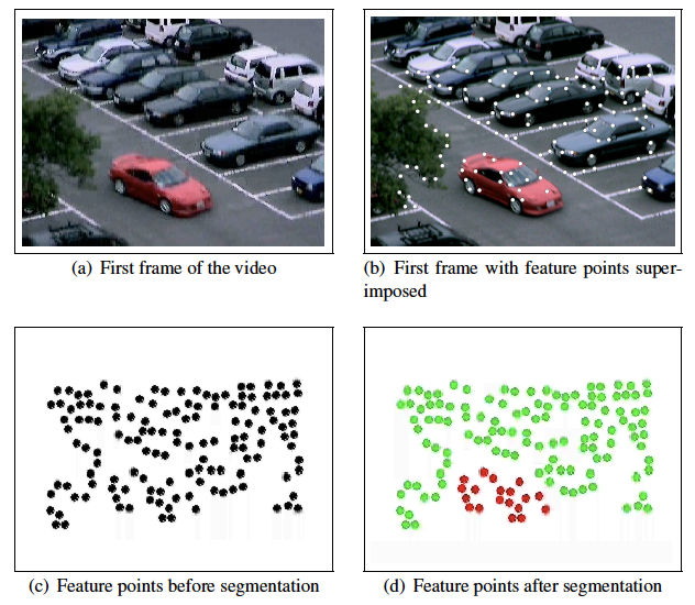
Even accounting for its elegance and simplicity, the low-rank assumption is too restrictive to be broadly applicable to modeling real-world data. A key limitation is the assumption of a single linear subspace that is responsible for generating the structured observations. In many practical applications, structure generated by a mixture of distinct low-dimensional subspaces provides a more realistic model. For example, consider a video sequence that captures the motion of several distinct objects, each subject to its own independent displacement (Figure 2.3 left). Under suitable assumptions on the individual motions, each object becomes responsible for an independent low-dimensional subspace in the concatenated sequence of video frames [VM04]. As another example, consider modeling natural images via learning a model for the distribution of patches, spatially-contiguous collections of pixels, within an image (Figure 2.3 right). Unlike in the Eigenface example we saw previously, where images of faces with matched poses can be well-approximated by a single low-dimensional subspace, the patch at a specific location in a natural image can correspond to objects with very different properties—for example, distinct color or shape due to occlusion boundaries. Therefore, modeling the distribution of patches with a single subspace is futile, but a mixture of subspaces, one for each region, performs surprisingly well in practice, say for segmenting or compressing purposes [MRY+11].555We will return to this observation in Chapter 4, where we will show it can be significantly generalized to learn representations for large-scale modern datasets. We will see a concrete example in the next chapter (Example 3.12).

Figure 2.4 : Data on a mixture of low-dimensional subspaces, say 𝒮 j = col ( 𝑼 j ) \mathcal{S}_{j}=\mathop{\mathrm{col}}(\bm{U}_{j}) caligraphic_S start_POSTSUBSCRIPT italic_j end_POSTSUBSCRIPT = roman_col ( bold_italic_U start_POSTSUBSCRIPT italic_j end_POSTSUBSCRIPT ) .
Figure 2.4: Data on a mixture of low-dimensional subspaces, say 𝒮j=col(𝑼j)\mathcal{S}_{j}=\mathop{\mathrm{col}}(\bm{U}_{j})caligraphic_S start_POSTSUBSCRIPT italic_j end_POSTSUBSCRIPT = roman_col ( bold_italic_U start_POSTSUBSCRIPT italic_j end_POSTSUBSCRIPT ).

In this section, we will begin by discussing the conceptual and algorithmic foundations for structured representation learning when the data distribution can be modeled by a mixture of low-dimensional subspaces, as illustrated in Figure 2.4. In this setting, the decoder mapping will be almost as simple as the case of a single subspace: we simply represent via

𝒙^=𝒟(𝒛)=(k=1Kπk(𝒛)𝑼k)𝒛,\hat{\bm{x}}=\mathcal{D}(\bm{z})=\left(\sum_{k=1}^{K}\pi_{k}(\bm{z})\bm{U}_{k}\right)\bm{z},over^ start_ARG bold_italic_x end_ARG = caligraphic_D ( bold_italic_z ) = ( ∑ start_POSTSUBSCRIPT italic_k = 1 end_POSTSUBSCRIPT start_POSTSUPERSCRIPT italic_K end_POSTSUPERSCRIPT italic_π start_POSTSUBSCRIPT italic_k end_POSTSUBSCRIPT ( bold_italic_z ) bold_italic_U start_POSTSUBSCRIPT italic_k end_POSTSUBSCRIPT ) bold_italic_z , (2.2.1)

where πk:d{0,1}\pi_{k}:\mathbb{R}^{d}\to\{0,1\}italic_π start_POSTSUBSCRIPT italic_k end_POSTSUBSCRIPT : blackboard_R start_POSTSUPERSCRIPT italic_d end_POSTSUPERSCRIPT → { 0 , 1 } are a set of sparse weighting random variables, such that only a single subspace 𝒮k=col(𝑼k)\mathcal{S}_{k}=\mathop{\mathrm{col}}(\bm{U}_{k})caligraphic_S start_POSTSUBSCRIPT italic_k end_POSTSUBSCRIPT = roman_col ( bold_italic_U start_POSTSUBSCRIPT italic_k end_POSTSUBSCRIPT ) is selected in the sum. However, the task of encoding such data 𝒙\bm{x}bold_italic_x to suitable representations 𝒛\bm{z}bold_italic_z, and learning such an encoder-decoder pair from data, will prove to be more involved.

We will see how ideas from the rich literature on sparse representation and independent component analysis lead to a natural reformulation of the above decoder architecture through the lens of sparsity, the corresponding encoder architecture (obtained through a power-method-like algorithm analogous to that of principal component analysis), and strong guarantees of correctness and efficiency for learning such encoder-decoder pairs from data. In this sense, the case of mixed linear low-dimensional structure already leads to many of the key conceptual components of structured representation learning that we will develop in far greater generality in this book.

2.2.1 Mixtures of Subspaces and Sparsely-Used Dictionaries

Let 𝑼1,,𝑼K\bm{U}_{1},\dots,\bm{U}_{K}bold_italic_U start_POSTSUBSCRIPT 1 end_POSTSUBSCRIPT , … , bold_italic_U start_POSTSUBSCRIPT italic_K end_POSTSUBSCRIPT, each of size D×dD\times ditalic_D × italic_d, denote a collection of orthonormal bases for KKitalic_K subspaces of dimension dditalic_d in D\mathbb{R}^{D}blackboard_R start_POSTSUPERSCRIPT italic_D end_POSTSUPERSCRIPT. To say that 𝒙\bm{x}bold_italic_x follows a mixture-of-subspaces distribution parameterized by 𝑼1,,𝑼K\bm{U}_{1},\dots,\bm{U}_{K}bold_italic_U start_POSTSUBSCRIPT 1 end_POSTSUBSCRIPT , … , bold_italic_U start_POSTSUBSCRIPT italic_K end_POSTSUBSCRIPT means, geometrically speaking, that

𝒙=𝑼k𝒛for somek[K],𝒛d.\bm{x}=\bm{U}_{k}\bm{z}\quad\text{for some}\enspace k\in[K],\enspace\bm{z}\in\mathbb{R}^{d}.bold_italic_x = bold_italic_U start_POSTSUBSCRIPT italic_k end_POSTSUBSCRIPT bold_italic_z for some italic_k ∈ [ italic_K ] , bold_italic_z ∈ blackboard_R start_POSTSUPERSCRIPT italic_d end_POSTSUPERSCRIPT . (2.2.2)

The statistical analogue of this geometric model, as we saw for the case of PCA and linear structure, is that 𝒙\bm{x}bold_italic_x follows a mixture of Gaussians distribution: that is,

𝒙k=1Kπk𝒩(𝟎,𝑼k𝑼k),for someπk0,k=1Kπk=1.\bm{x}\sim\sum_{k=1}^{K}\pi_{k}\mathcal{N}(\mathbf{0},\bm{U}_{k}\bm{U}_{k}^{\top}),\quad\text{for some}\enspace\pi_{k}\geq 0,\enspace\sum_{k=1}^{K}\pi_{k}=1.bold_italic_x ∼ ∑ start_POSTSUBSCRIPT italic_k = 1 end_POSTSUBSCRIPT start_POSTSUPERSCRIPT italic_K end_POSTSUPERSCRIPT italic_π start_POSTSUBSCRIPT italic_k end_POSTSUBSCRIPT caligraphic_N ( bold_0 , bold_italic_U start_POSTSUBSCRIPT italic_k end_POSTSUBSCRIPT bold_italic_U start_POSTSUBSCRIPT italic_k end_POSTSUBSCRIPT start_POSTSUPERSCRIPT ⊤ end_POSTSUPERSCRIPT ) , for some italic_π start_POSTSUBSCRIPT italic_k end_POSTSUBSCRIPT ≥ 0 , ∑ start_POSTSUBSCRIPT italic_k = 1 end_POSTSUBSCRIPT start_POSTSUPERSCRIPT italic_K end_POSTSUPERSCRIPT italic_π start_POSTSUBSCRIPT italic_k end_POSTSUBSCRIPT = 1 . (2.2.3)

In other words, for each k[K]k\in[K]italic_k ∈ [ italic_K ], 𝒙\bm{x}bold_italic_x is Gaussian on the low-dimensional subspace col(𝑼k)\mathop{\mathrm{col}}(\bm{U}_{k})roman_col ( bold_italic_U start_POSTSUBSCRIPT italic_k end_POSTSUBSCRIPT ) with probability πk\pi_{k}italic_π start_POSTSUBSCRIPT italic_k end_POSTSUBSCRIPT.

Remark 2.6 (A Mixture of Gaussians v.s. A Superposition of Gaussians).

One should be aware that the above model (2.2.3) is a mixture of Gaussian distributions, not to be confused with a mixture of Gaussian variables by superposition, say

𝒙=i=1nwi𝒙i,𝒙i𝒩(𝟎,𝑼i𝑼i),\bm{x}=\sum_{i=1}^{n}w_{i}\bm{x}_{i},\quad\bm{x}_{i}\sim\mathcal{N}(\mathbf{0},\bm{U}_{i}\bm{U}_{i}^{\top}),bold_italic_x = ∑ start_POSTSUBSCRIPT italic_i = 1 end_POSTSUBSCRIPT start_POSTSUPERSCRIPT italic_n end_POSTSUPERSCRIPT italic_w start_POSTSUBSCRIPT italic_i end_POSTSUBSCRIPT bold_italic_x start_POSTSUBSCRIPT italic_i end_POSTSUBSCRIPT , bold_italic_x start_POSTSUBSCRIPT italic_i end_POSTSUBSCRIPT ∼ caligraphic_N ( bold_0 , bold_italic_U start_POSTSUBSCRIPT italic_i end_POSTSUBSCRIPT bold_italic_U start_POSTSUBSCRIPT italic_i end_POSTSUBSCRIPT start_POSTSUPERSCRIPT ⊤ end_POSTSUPERSCRIPT ) , (2.2.4)

where 𝒙i\bm{x}_{i}bold_italic_x start_POSTSUBSCRIPT italic_i end_POSTSUBSCRIPT are independent random Gaussian vectors and wiw_{i}italic_w start_POSTSUBSCRIPT italic_i end_POSTSUBSCRIPT are a set of fixed weights. As we know from the properties of Gaussian vectors, such a superposition 𝒙\bm{x}bold_italic_x will remain a Gaussian distribution.

For now, we focus on the geometric perspective offered by (2.2.2). There is an algebraically convenient alternative to this conditional representation. Consider a lifted representation vector 𝒛=[𝒛1,,𝒛K]dK\bm{z}=[\bm{z}_{1}^{\top},\dots,\bm{z}_{K}^{\top}]^{\top}\in\mathbb{R}^{dK}bold_italic_z = [ bold_italic_z start_POSTSUBSCRIPT 1 end_POSTSUBSCRIPT start_POSTSUPERSCRIPT ⊤ end_POSTSUPERSCRIPT , … , bold_italic_z start_POSTSUBSCRIPT italic_K end_POSTSUBSCRIPT start_POSTSUPERSCRIPT ⊤ end_POSTSUPERSCRIPT ] start_POSTSUPERSCRIPT ⊤ end_POSTSUPERSCRIPT ∈ blackboard_R start_POSTSUPERSCRIPT italic_d italic_K end_POSTSUPERSCRIPT, such that 𝒛\bm{z}bold_italic_z is dditalic_d-sparse with support on one of the KKitalic_K consecutive non-overlapping blocks of dditalic_d coordinates out of dKdKitalic_d italic_K. Then (2.2.2) can be written equivalently as

𝒙=[||𝑼1𝑼K||]𝑼[𝒛1𝒛K]𝒛,[𝒛12𝒛K2]0=1.\bm{x}=\underbrace{\begin{bmatrix}|&\ldots&|\\ \bm{U}_{1}&\ldots&\bm{U}_{K}\\ |&\ldots&|\end{bmatrix}}_{\bm{U}}\underbrace{\begin{bmatrix}\bm{z}_{1}\\ \vdots\\ \bm{z}_{K}\end{bmatrix}}_{\bm{z}},\quad\left\|\begin{bmatrix}\left\|\bm{z}_{1}\right\|_{2}\\ \vdots\\ \left\|\bm{z}_{K}\right\|_{2}\end{bmatrix}\right\|_{0}=1.bold_italic_x = under⏟ start_ARG [ start_ARG start_ROW start_CELL | end_CELL start_CELL … end_CELL start_CELL | end_CELL end_ROW start_ROW start_CELL bold_italic_U start_POSTSUBSCRIPT 1 end_POSTSUBSCRIPT end_CELL start_CELL … end_CELL start_CELL bold_italic_U start_POSTSUBSCRIPT italic_K end_POSTSUBSCRIPT end_CELL end_ROW start_ROW start_CELL | end_CELL start_CELL … end_CELL start_CELL | end_CELL end_ROW end_ARG ] end_ARG start_POSTSUBSCRIPT bold_italic_U end_POSTSUBSCRIPT under⏟ start_ARG [ start_ARG start_ROW start_CELL bold_italic_z start_POSTSUBSCRIPT 1 end_POSTSUBSCRIPT end_CELL end_ROW start_ROW start_CELL ⋮ end_CELL end_ROW start_ROW start_CELL bold_italic_z start_POSTSUBSCRIPT italic_K end_POSTSUBSCRIPT end_CELL end_ROW end_ARG ] end_ARG start_POSTSUBSCRIPT bold_italic_z end_POSTSUBSCRIPT , ∥ [ start_ARG start_ROW start_CELL ∥ bold_italic_z start_POSTSUBSCRIPT 1 end_POSTSUBSCRIPT ∥ start_POSTSUBSCRIPT 2 end_POSTSUBSCRIPT end_CELL end_ROW start_ROW start_CELL ⋮ end_CELL end_ROW start_ROW start_CELL ∥ bold_italic_z start_POSTSUBSCRIPT italic_K end_POSTSUBSCRIPT ∥ start_POSTSUBSCRIPT 2 end_POSTSUBSCRIPT end_CELL end_ROW end_ARG ] ∥ start_POSTSUBSCRIPT 0 end_POSTSUBSCRIPT = 1 . (2.2.5)

Here, the 0\ell^{0}roman_ℓ start_POSTSUPERSCRIPT 0 end_POSTSUPERSCRIPT “norm” 0\|\,\cdot\,\|_{0}∥ ⋅ ∥ start_POSTSUBSCRIPT 0 end_POSTSUBSCRIPT measures sparsity by counting the number of nonzero entries:

𝒛0=|{izi0}|,\|\bm{z}\|_{0}=\left\lvert\{i\mid z_{i}\neq 0\}\right\rvert,∥ bold_italic_z ∥ start_POSTSUBSCRIPT 0 end_POSTSUBSCRIPT = | { italic_i ∣ italic_z start_POSTSUBSCRIPT italic_i end_POSTSUBSCRIPT ≠ 0 } | , (2.2.6)

and the matrix 𝑼D×Kd\bm{U}\in\mathbb{R}^{D\times Kd}bold_italic_U ∈ blackboard_R start_POSTSUPERSCRIPT italic_D × italic_K italic_d end_POSTSUPERSCRIPT is called a dictionary with all the {𝑼i}i=1K\{\bm{U}_{i}\}_{i=1}^{K}{ bold_italic_U start_POSTSUBSCRIPT italic_i end_POSTSUBSCRIPT } start_POSTSUBSCRIPT italic_i = 1 end_POSTSUBSCRIPT start_POSTSUPERSCRIPT italic_K end_POSTSUPERSCRIPT as code words. In general, if the number of subspaces in the mixture KKitalic_K is large enough, there is no bound on the number of columns contained in the dictionary 𝑼\bm{U}bold_italic_U. In the case where Kd<DKd<Ditalic_K italic_d < italic_D, 𝑼\bm{U}bold_italic_U is called undercomplete; when Kd=DKd=Ditalic_K italic_d = italic_D, it is called complete; and when Kd>DKd>Ditalic_K italic_d > italic_D, it is called overcomplete.

Now, (2.2.5) suggests a convenient relaxation for tractability of analysis: rather than modeling 𝒙\bm{x}bold_italic_x as coming from a mixture of KKitalic_K specific subspaces 𝑼1,,𝑼K\bm{U}_{1},\dots,\bm{U}_{K}bold_italic_U start_POSTSUBSCRIPT 1 end_POSTSUBSCRIPT , … , bold_italic_U start_POSTSUBSCRIPT italic_K end_POSTSUBSCRIPT, we may instead start with a dictionary 𝑼D×m\bm{U}\in\mathbb{R}^{D\times m}bold_italic_U ∈ blackboard_R start_POSTSUPERSCRIPT italic_D × italic_m end_POSTSUPERSCRIPT, where mmitalic_m may be smaller or larger than DDitalic_D, and simply seek to represent 𝒙=𝑼𝒛\bm{x}=\bm{U}\bm{z}bold_italic_x = bold_italic_U bold_italic_z with the sparsity 𝒛0\|\bm{z}\|_{0}∥ bold_italic_z ∥ start_POSTSUBSCRIPT 0 end_POSTSUBSCRIPT sufficiently small. This leads to the sparse dictionary model for 𝒙\bm{x}bold_italic_x:

𝒙=𝑼𝒛+𝜺,𝒛0d,\bm{x}=\bm{U}\bm{z}+\bm{\varepsilon},\quad\|\bm{z}\|_{0}\ll d,bold_italic_x = bold_italic_U bold_italic_z + bold_italic_ε , ∥ bold_italic_z ∥ start_POSTSUBSCRIPT 0 end_POSTSUBSCRIPT ≪ italic_d , (2.2.7)

where 𝜺\bm{\varepsilon}bold_italic_ε represents an unknown noise vector. Geometrically, this implies that 𝒙\bm{x}bold_italic_x lies close to the span of a subset of 𝒛0\|\bm{z}\|_{0}∥ bold_italic_z ∥ start_POSTSUBSCRIPT 0 end_POSTSUBSCRIPT columns of 𝑼\bm{U}bold_italic_U, making this an instantiation of the mixture-of-subspaces model (2.2.2) with a very large value of KKitalic_K, and specific correlations between the subspaces 𝑼k\bm{U}_{k}bold_italic_U start_POSTSUBSCRIPT italic_k end_POSTSUBSCRIPT.

Orthogonal dictionary for sparse coding.

Now we can formulate the structured representation learning problem for mixtures of low-dimensional subspaces that we will study in this section. We assume that we have samples 𝑿=[𝒙1,,𝒙N]\bm{X}=[\bm{x}_{1},\dots,\bm{x}_{N}]bold_italic_X = [ bold_italic_x start_POSTSUBSCRIPT 1 end_POSTSUBSCRIPT , … , bold_italic_x start_POSTSUBSCRIPT italic_N end_POSTSUBSCRIPT ] from an unknown sparse dictionary model (2.2.7), possibly with added noises 𝜺i\bm{\varepsilon}_{i}bold_italic_ε start_POSTSUBSCRIPT italic_i end_POSTSUBSCRIPT. Let us begin from the assumption that the dictionary 𝑼\bm{U}bold_italic_U in the sparse dictionary model (2.2.7) is complete and orthogonal,666It can be shown that for the complete case, we do not lose any generality by making the orthogonal assumption (Exercise 2.4). and that each coefficient vector 𝒛\bm{z}bold_italic_z is dditalic_d-sparse, with dDd\ll Ditalic_d ≪ italic_D. In this setting, representation learning amounts to correctly learning the orthogonal dictionary 𝑼\bm{U}bold_italic_U via optimization: we can then take (𝒙)=𝑼𝒙\mathcal{E}(\bm{x})=\bm{U}^{\top}\bm{x}caligraphic_E ( bold_italic_x ) = bold_italic_U start_POSTSUPERSCRIPT ⊤ end_POSTSUPERSCRIPT bold_italic_x as the encoder and 𝒟(𝒛)=𝑼𝒛\mathcal{D}(\bm{z})=\bm{U}\bm{z}caligraphic_D ( bold_italic_z ) = bold_italic_U bold_italic_z as the decoder, and 𝒟=1\mathcal{D}=\mathcal{E}^{-1}caligraphic_D = caligraphic_E start_POSTSUPERSCRIPT - 1 end_POSTSUPERSCRIPT. In diagram form:

𝒙=𝑼𝒛𝒟=𝑼𝒙^.\bm{x}\xrightarrow{\hskip 5.69054pt\mathcal{E}=\bm{U}^{\top}\hskip 5.69054pt}\bm{z}\xrightarrow{\hskip 5.69054pt\mathcal{D}=\bm{U}\hskip 5.69054pt}\hat{\bm{x}}.bold_italic_x start_ARROW start_OVERACCENT caligraphic_E = bold_italic_U start_POSTSUPERSCRIPT ⊤ end_POSTSUPERSCRIPT end_OVERACCENT → end_ARROW bold_italic_z start_ARROW start_OVERACCENT caligraphic_D = bold_italic_U end_OVERACCENT → end_ARROW over^ start_ARG bold_italic_x end_ARG . (2.2.8)

We see that the autoencoding pair (,𝒟)(\mathcal{E},\mathcal{D})( caligraphic_E , caligraphic_D ) for complete dictionary learning is symmetric, as in the case of a single linear subspace, making the computational task of encoding and decoding no more difficult than in the linear case. On the other hand, the task of learning the dictionary 𝑼\bm{U}bold_italic_U is strictly more difficult than learning a single linear subspace by PCA. To see why we cannot simply use PCA to learn the orthogonal dictionary 𝑼\bm{U}bold_italic_U correctly, note that the loss function that gave rise to PCA, namely (2.1.5), is completely invariant to rotations of the rows of the matrix 𝑼\bm{U}bold_italic_U: that is, if 𝑸\bm{Q}bold_italic_Q is any d×dd\times ditalic_d × italic_d orthogonal matrix, then 𝑼\bm{U}bold_italic_U and 𝑼𝑸\bm{U}\bm{Q}bold_italic_U bold_italic_Q are both feasible and have an identical loss for (2.1.5). The sparse dictionary model is decidedly not invariant to such transformations: if we replaced 𝑼\bm{U}bold_italic_U by 𝑼𝑸\bm{U}\bm{Q}bold_italic_U bold_italic_Q and made a corresponding rotation 𝑸𝒛\bm{Q}^{\top}\bm{z}bold_italic_Q start_POSTSUPERSCRIPT ⊤ end_POSTSUPERSCRIPT bold_italic_z of the representation coefficients 𝒛\bm{z}bold_italic_z, we would in general destroy the sparsity structure of 𝒛\bm{z}bold_italic_z, violating the modeling assumption. Thus, we need new algorithms for learning orthogonal dictionaries.

2.2.2 Complete Dictionary Learning

In this section, we will derive algorithms for solving the orthogonal dictionary learning problem. To be more precise, we assume that the observed vector 𝒙D\bm{x}\in\mathbb{R}^{D}bold_italic_x ∈ blackboard_R start_POSTSUPERSCRIPT italic_D end_POSTSUPERSCRIPT follows a statistical model

𝒙=𝑼𝒛+𝜺,\bm{x}=\bm{U}\bm{z}+\bm{\varepsilon},bold_italic_x = bold_italic_U bold_italic_z + bold_italic_ε , (2.2.9)

where 𝑼D×D\bm{U}\in\mathbb{R}^{D\times D}bold_italic_U ∈ blackboard_R start_POSTSUPERSCRIPT italic_D × italic_D end_POSTSUPERSCRIPT is an unknown orthogonal dictionary, 𝒛\bm{z}bold_italic_z is a random vector with statistically independent components ziz_{i}italic_z start_POSTSUBSCRIPT italic_i end_POSTSUBSCRIPT, each with zero mean, and 𝜺D\bm{\varepsilon}\in\mathbb{R}^{D}bold_italic_ε ∈ blackboard_R start_POSTSUPERSCRIPT italic_D end_POSTSUPERSCRIPT is an independent random vector of small (Gaussian) noises. The goal is to recover 𝑼\bm{U}bold_italic_U (and hence 𝒛\bm{z}bold_italic_z) from samples of 𝒙\bm{x}bold_italic_x.

Here we assume that each independent component ziz_{i}italic_z start_POSTSUBSCRIPT italic_i end_POSTSUBSCRIPT is distributed as

ziBern(θ)𝒩(0,1/θ).z_{i}\sim\mathrm{Bern}(\theta)\cdot\mathcal{N}(0,1/\theta).italic_z start_POSTSUBSCRIPT italic_i end_POSTSUBSCRIPT ∼ roman_Bern ( italic_θ ) ⋅ caligraphic_N ( 0 , 1 / italic_θ ) .

That is, it is the product of a Bernoulli random variable with probability θ\thetaitalic_θ of being 111 and 1θ1-\theta1 - italic_θ of being 0, and an independent Gaussian random variable with variance 1/θ1/\theta1 / italic_θ. This distribution is formally known as the Bernoulli-Gaussian distribution. The normalization is chosen so that Var(zi)=1\operatorname{Var}(z_{i})=1roman_Var ( italic_z start_POSTSUBSCRIPT italic_i end_POSTSUBSCRIPT ) = 1 and hence 𝔼[𝒛22]=d\mathbb{E}[\|\bm{z}\|_{2}^{2}]=dblackboard_E [ ∥ bold_italic_z ∥ start_POSTSUBSCRIPT 2 end_POSTSUBSCRIPT start_POSTSUPERSCRIPT 2 end_POSTSUPERSCRIPT ] = italic_d. This modeling assumption implies that the vector of independent components 𝒛\bm{z}bold_italic_z is typically very sparse: we calculate 𝔼[𝒛0]=dθ\mathbb{E}\left[\|\bm{z}\|_{0}\right]=d\thetablackboard_E [ ∥ bold_italic_z ∥ start_POSTSUBSCRIPT 0 end_POSTSUBSCRIPT ] = italic_d italic_θ, which is small when θ\thetaitalic_θ is inversely proportional to dditalic_d.

Remark 2.7 (The Orthogonal Assumption).

At first sight, the assumption that the dictionary 𝑼\bm{U}bold_italic_U is orthogonal might seem to be somewhat restrictive. But there is actually no loss of generality. One may consider a complete dictionary to be any square invertible matrix 𝑼\bm{U}bold_italic_U. With samples generated from this dictionary: 𝑿=𝑼𝒁D×N\bm{X}=\bm{U}\bm{Z}\in\mathbb{R}^{D\times N}bold_italic_X = bold_italic_U bold_italic_Z ∈ blackboard_R start_POSTSUPERSCRIPT italic_D × italic_N end_POSTSUPERSCRIPT, it is easy to show that with some preconditioning of the data matrix 𝑿\bm{X}bold_italic_X:

𝑿¯=(1Nθ𝑿𝑿)12𝑿,\bar{\bm{X}}=\Big{(}\frac{1}{N\theta}\bm{X}\bm{X}^{\top}\Big{)}^{-\frac{1}{2}}\bm{X},over¯ start_ARG bold_italic_X end_ARG = ( divide start_ARG 1 end_ARG start_ARG italic_N italic_θ end_ARG bold_italic_X bold_italic_X start_POSTSUPERSCRIPT ⊤ end_POSTSUPERSCRIPT ) start_POSTSUPERSCRIPT - divide start_ARG 1 end_ARG start_ARG 2 end_ARG end_POSTSUPERSCRIPT bold_italic_X , (2.2.10)

then there exists an orthogonal matrix 𝑼o𝖮(D)\bm{U}_{o}\in\mathsf{O}(D)bold_italic_U start_POSTSUBSCRIPT italic_o end_POSTSUBSCRIPT ∈ sansserif_O ( italic_D ) such that

𝑿¯=𝑼o𝒁.\bar{\bm{X}}=\bm{U}_{o}\bm{Z}.over¯ start_ARG bold_italic_X end_ARG = bold_italic_U start_POSTSUBSCRIPT italic_o end_POSTSUBSCRIPT bold_italic_Z . (2.2.11)

See Exercise 2.4 or [SQW17a] for more details.

Figure 2.5 : Maximizing ℓ 4 \ell^{4} roman_ℓ start_POSTSUPERSCRIPT 4 end_POSTSUPERSCRIPT norm or minimizing ℓ 1 \ell^{1} roman_ℓ start_POSTSUPERSCRIPT 1 end_POSTSUPERSCRIPT norm promotes sparsity (for vectors on the sphere).
Figure 2.5: Maximizing 4\ell^{4}roman_ℓ start_POSTSUPERSCRIPT 4 end_POSTSUPERSCRIPT norm or minimizing 1\ell^{1}roman_ℓ start_POSTSUPERSCRIPT 1 end_POSTSUPERSCRIPT norm promotes sparsity (for vectors on the sphere).

Dictionary learning via the MSP algorithm.

Now suppose that we are given a set of observations:

𝒙i=𝑼𝒛i+𝜺i,i[N].\bm{x}_{i}=\bm{U}\bm{z}_{i}+\bm{\varepsilon}_{i},\ \forall i\in[N].bold_italic_x start_POSTSUBSCRIPT italic_i end_POSTSUBSCRIPT = bold_italic_U bold_italic_z start_POSTSUBSCRIPT italic_i end_POSTSUBSCRIPT + bold_italic_ε start_POSTSUBSCRIPT italic_i end_POSTSUBSCRIPT , ∀ italic_i ∈ [ italic_N ] . (2.2.12)

Let 𝑿=[𝒙1,,𝒙N]\bm{X}=[\bm{x}_{1},\dots,\bm{x}_{N}]bold_italic_X = [ bold_italic_x start_POSTSUBSCRIPT 1 end_POSTSUBSCRIPT , … , bold_italic_x start_POSTSUBSCRIPT italic_N end_POSTSUBSCRIPT ] and 𝒁=[𝒛1,,𝒛N]\bm{Z}=[\bm{z}_{1},\dots,\bm{z}_{N}]bold_italic_Z = [ bold_italic_z start_POSTSUBSCRIPT 1 end_POSTSUBSCRIPT , … , bold_italic_z start_POSTSUBSCRIPT italic_N end_POSTSUBSCRIPT ]. The goal is to recover 𝑼\bm{U}bold_italic_U from the data 𝑿\bm{X}bold_italic_X. Therefore, given any orthogonal matrix 𝑨𝖮(D)\bm{A}\in\mathsf{O}(D)bold_italic_A ∈ sansserif_O ( italic_D ),

𝑨𝒙i=𝑨𝑼𝒛i+𝑨𝜺i\bm{A}\bm{x}_{i}=\bm{A}\bm{U}\bm{z}_{i}+\bm{A}\bm{\varepsilon}_{i}bold_italic_A bold_italic_x start_POSTSUBSCRIPT italic_i end_POSTSUBSCRIPT = bold_italic_A bold_italic_U bold_italic_z start_POSTSUBSCRIPT italic_i end_POSTSUBSCRIPT + bold_italic_A bold_italic_ε start_POSTSUBSCRIPT italic_i end_POSTSUBSCRIPT (2.2.13)

would be nearly sparse if 𝑨=𝑼T\bm{A}=\bm{U}^{T}bold_italic_A = bold_italic_U start_POSTSUPERSCRIPT italic_T end_POSTSUPERSCRIPT (as by assumption the noise 𝜺i\bm{\varepsilon}_{i}bold_italic_ε start_POSTSUBSCRIPT italic_i end_POSTSUBSCRIPT is of small magnitude).

Also, given 𝑼\bm{U}bold_italic_U is orthogonal and the fact 𝜺\bm{\varepsilon}bold_italic_ε is small, the vector 𝒙\bm{x}bold_italic_x has a predictable expected norm, i.e., 𝔼[𝒙22]𝔼[𝒛22]=d\mathbb{E}[\|\bm{x}\|_{2}^{2}]\approx\mathbb{E}[\|\bm{z}\|_{2}^{2}]=dblackboard_E [ ∥ bold_italic_x ∥ start_POSTSUBSCRIPT 2 end_POSTSUBSCRIPT start_POSTSUPERSCRIPT 2 end_POSTSUPERSCRIPT ] ≈ blackboard_E [ ∥ bold_italic_z ∥ start_POSTSUBSCRIPT 2 end_POSTSUBSCRIPT start_POSTSUPERSCRIPT 2 end_POSTSUPERSCRIPT ] = italic_d. It is a known fact that for vectors on a sphere, maximizing the 4\ell^{4}roman_ℓ start_POSTSUPERSCRIPT 4 end_POSTSUPERSCRIPT norm is equivalent to minimizing the 0\ell^{0}roman_ℓ start_POSTSUPERSCRIPT 0 end_POSTSUPERSCRIPT norm (for promoting sparsity),

argmax𝒛𝕊n𝒛4argmin𝒛𝕊n𝒛0.\operatorname*{arg\ max}_{\bm{z}\in\mathbb{S}^{n}}\|\bm{z}\|_{4}\quad\Leftrightarrow\quad\operatorname*{arg\ min}_{\bm{z}\in\mathbb{S}^{n}}\|\bm{z}\|_{0}.start_OPERATOR roman_arg roman_max end_OPERATOR start_POSTSUBSCRIPT bold_italic_z ∈ blackboard_S start_POSTSUPERSCRIPT italic_n end_POSTSUPERSCRIPT end_POSTSUBSCRIPT ∥ bold_italic_z ∥ start_POSTSUBSCRIPT 4 end_POSTSUBSCRIPT ⇔ start_OPERATOR roman_arg roman_min end_OPERATOR start_POSTSUBSCRIPT bold_italic_z ∈ blackboard_S start_POSTSUPERSCRIPT italic_n end_POSTSUPERSCRIPT end_POSTSUBSCRIPT ∥ bold_italic_z ∥ start_POSTSUBSCRIPT 0 end_POSTSUBSCRIPT . (2.2.14)

This is illustrated in Figure 2.5.

An orthogonal matrix 𝑨\bm{A}bold_italic_A preserves the Euclidean (2\ell^{2}roman_ℓ start_POSTSUPERSCRIPT 2 end_POSTSUPERSCRIPT) norm: 𝑨𝒙22=𝒙22\|\bm{A}\bm{x}\|_{2}^{2}=\|\bm{x}\|_{2}^{2}∥ bold_italic_A bold_italic_x ∥ start_POSTSUBSCRIPT 2 end_POSTSUBSCRIPT start_POSTSUPERSCRIPT 2 end_POSTSUPERSCRIPT = ∥ bold_italic_x ∥ start_POSTSUBSCRIPT 2 end_POSTSUBSCRIPT start_POSTSUPERSCRIPT 2 end_POSTSUPERSCRIPT. Therefore, to find the correct orthogonal dictionary 𝑼\bm{U}bold_italic_U from 𝑿\bm{X}bold_italic_X, we may try to solve the following optimization program:

max𝑨~𝖮(D)14𝑨~𝑿44=14i=1N𝑨~𝒙i44\max_{\tilde{\bm{A}}\in\mathsf{O}(D)}\,\frac{1}{4}\left\|\tilde{\bm{A}}\bm{X}\right\|_{4}^{4}=\frac{1}{4}\sum_{i=1}^{N}\left\|\tilde{\bm{A}}\bm{x}_{i}\right\|_{4}^{4}roman_max start_POSTSUBSCRIPT over~ start_ARG bold_italic_A end_ARG ∈ sansserif_O ( italic_D ) end_POSTSUBSCRIPT divide start_ARG 1 end_ARG start_ARG 4 end_ARG ∥ over~ start_ARG bold_italic_A end_ARG bold_italic_X ∥ start_POSTSUBSCRIPT 4 end_POSTSUBSCRIPT start_POSTSUPERSCRIPT 4 end_POSTSUPERSCRIPT = divide start_ARG 1 end_ARG start_ARG 4 end_ARG ∑ start_POSTSUBSCRIPT italic_i = 1 end_POSTSUBSCRIPT start_POSTSUPERSCRIPT italic_N end_POSTSUPERSCRIPT ∥ over~ start_ARG bold_italic_A end_ARG bold_italic_x start_POSTSUBSCRIPT italic_i end_POSTSUBSCRIPT ∥ start_POSTSUBSCRIPT 4 end_POSTSUBSCRIPT start_POSTSUPERSCRIPT 4 end_POSTSUPERSCRIPT (2.2.15)

This is known as the 4\ell^{4}roman_ℓ start_POSTSUPERSCRIPT 4 end_POSTSUPERSCRIPT maximization problem [ZMZ+20]. After we find the solution 𝑨\bm{A}^{\star}bold_italic_A start_POSTSUPERSCRIPT ⋆ end_POSTSUPERSCRIPT, we can take the transpose 𝑼=(𝑨)\bm{U}^{\star}=(\bm{A}^{\star})^{\top}bold_italic_U start_POSTSUPERSCRIPT ⋆ end_POSTSUPERSCRIPT = ( bold_italic_A start_POSTSUPERSCRIPT ⋆ end_POSTSUPERSCRIPT ) start_POSTSUPERSCRIPT ⊤ end_POSTSUPERSCRIPT.

Remark 2.8.

It is also known that for vectors on a sphere, minimizing the 1\ell^{1}roman_ℓ start_POSTSUPERSCRIPT 1 end_POSTSUPERSCRIPT norm is equivalent to minimizing the 0\ell^{0}roman_ℓ start_POSTSUPERSCRIPT 0 end_POSTSUPERSCRIPT norm (for promoting sparsity),

argmin𝒛𝕊n𝒛1argmin𝒛𝕊n𝒛0,\operatorname*{arg\ min}_{\bm{z}\in\mathbb{S}^{n}}\|\bm{z}\|_{1}\quad\Leftrightarrow\quad\operatorname*{arg\ min}_{\bm{z}\in\mathbb{S}^{n}}\|\bm{z}\|_{0},start_OPERATOR roman_arg roman_min end_OPERATOR start_POSTSUBSCRIPT bold_italic_z ∈ blackboard_S start_POSTSUPERSCRIPT italic_n end_POSTSUPERSCRIPT end_POSTSUBSCRIPT ∥ bold_italic_z ∥ start_POSTSUBSCRIPT 1 end_POSTSUBSCRIPT ⇔ start_OPERATOR roman_arg roman_min end_OPERATOR start_POSTSUBSCRIPT bold_italic_z ∈ blackboard_S start_POSTSUPERSCRIPT italic_n end_POSTSUPERSCRIPT end_POSTSUBSCRIPT ∥ bold_italic_z ∥ start_POSTSUBSCRIPT 0 end_POSTSUBSCRIPT ,

which is also illustrated in Figure 2.5. This fact can also be exploited to learn the dictionary 𝑨\bm{A}bold_italic_A effectively and efficiently. This was actually explored earlier than the 4\ell^{4}roman_ℓ start_POSTSUPERSCRIPT 4 end_POSTSUPERSCRIPT norm used here. Interested readers may refer to the work of [QZL+20a].

Note that the above problem is equivalent to the following constrained optimization problem:

min14𝑨~𝑿44subject to𝑨~𝑨~=𝑰.\min\,-\frac{1}{4}\left\|\tilde{\bm{A}}\bm{X}\right\|_{4}^{4}\quad\mbox{subject to}\quad\tilde{\bm{A}}^{\top}\tilde{\bm{A}}=\bm{I}.roman_min - divide start_ARG 1 end_ARG start_ARG 4 end_ARG ∥ over~ start_ARG bold_italic_A end_ARG bold_italic_X ∥ start_POSTSUBSCRIPT 4 end_POSTSUBSCRIPT start_POSTSUPERSCRIPT 4 end_POSTSUPERSCRIPT subject to over~ start_ARG bold_italic_A end_ARG start_POSTSUPERSCRIPT ⊤ end_POSTSUPERSCRIPT over~ start_ARG bold_italic_A end_ARG = bold_italic_I . (2.2.16)

As shown in [WM22], using the Lagrange multiplier method, one can derive that the optimal solution to the problem should satisfy the following “fixed point” condition:

𝑨=𝒫O(D)[(𝑨𝑿)3𝑿],\bm{A}^{\star}=\mathcal{P}_{\mathrm{O}(D)}[({\bm{A}^{\star}\bm{X}})^{\mathbin{\mathchoice{\raisebox{1.3pt}{$\displaystyle\mathchoice{\scalebox{0.8}{$\displaystyle\odot$}}{\scalebox{0.8}{$\textstyle\odot$}}{\scalebox{0.8}{$\scriptstyle\odot$}}{\scalebox{0.8}{$\scriptscriptstyle\odot$}}$}}{\raisebox{1.3pt}{$\mathchoice{\scalebox{0.8}{$\displaystyle\odot$}}{\scalebox{0.8}{$\textstyle\odot$}}{\scalebox{0.8}{$\scriptstyle\odot$}}{\scalebox{0.8}{$\scriptscriptstyle\odot$}}$}}{\raisebox{0.75pt}{$\scriptstyle\mathchoice{\scalebox{0.8}{$\displaystyle\odot$}}{\scalebox{0.8}{$\textstyle\odot$}}{\scalebox{0.8}{$\scriptstyle\odot$}}{\scalebox{0.8}{$\scriptscriptstyle\odot$}}$}}{\raisebox{0.6pt}{$\scriptscriptstyle\mathchoice{\scalebox{0.8}{$\displaystyle\odot$}}{\scalebox{0.8}{$\textstyle\odot$}}{\scalebox{0.8}{$\scriptstyle\odot$}}{\scalebox{0.8}{$\scriptscriptstyle\odot$}}$}}}3}\bm{X}^{\top}],bold_italic_A start_POSTSUPERSCRIPT ⋆ end_POSTSUPERSCRIPT = caligraphic_P start_POSTSUBSCRIPT roman_O ( italic_D ) end_POSTSUBSCRIPT [ ( bold_italic_A start_POSTSUPERSCRIPT ⋆ end_POSTSUPERSCRIPT bold_italic_X ) start_POSTSUPERSCRIPT ⊙ 3 end_POSTSUPERSCRIPT bold_italic_X start_POSTSUPERSCRIPT ⊤ end_POSTSUPERSCRIPT ] , (2.2.17)

where 𝒫O(D)[]\mathcal{P}_{\mathrm{O}(D)}[\,\cdot\,]caligraphic_P start_POSTSUBSCRIPT roman_O ( italic_D ) end_POSTSUBSCRIPT [ ⋅ ] is a projection onto the space of orthogonal matrices O(D)\mathrm{O}(D)roman_O ( italic_D ).777For any matrix 𝑴\bm{M}bold_italic_M with SVD 𝑴=𝑼𝚺𝑽\bm{M}=\bm{U}\bm{\Sigma}\bm{V}^{\top}bold_italic_M = bold_italic_U bold_Σ bold_italic_V start_POSTSUPERSCRIPT ⊤ end_POSTSUPERSCRIPT, 𝒫O(D)[𝑴]=𝑼𝑽\mathcal{P}_{\mathrm{O}(D)}[\bm{M}]=\bm{U}\bm{V}^{\top}caligraphic_P start_POSTSUBSCRIPT roman_O ( italic_D ) end_POSTSUBSCRIPT [ bold_italic_M ] = bold_italic_U bold_italic_V start_POSTSUPERSCRIPT ⊤ end_POSTSUPERSCRIPT. We leave this as an exercise for the reader.

To compute the fixed point for the above equation, similar to how we computed eigenvectors for PCA (2.1.16), we may take the following power iteration:

𝑨t+1=𝒫O(D)[(𝑨t𝑿)3𝑿].\bm{A}_{t+1}=\mathcal{P}_{\mathrm{O}(D)}[({\bm{A}_{t}\bm{X}})^{\mathbin{\mathchoice{\raisebox{1.3pt}{$\displaystyle\mathchoice{\scalebox{0.8}{$\displaystyle\odot$}}{\scalebox{0.8}{$\textstyle\odot$}}{\scalebox{0.8}{$\scriptstyle\odot$}}{\scalebox{0.8}{$\scriptscriptstyle\odot$}}$}}{\raisebox{1.3pt}{$\mathchoice{\scalebox{0.8}{$\displaystyle\odot$}}{\scalebox{0.8}{$\textstyle\odot$}}{\scalebox{0.8}{$\scriptstyle\odot$}}{\scalebox{0.8}{$\scriptscriptstyle\odot$}}$}}{\raisebox{0.75pt}{$\scriptstyle\mathchoice{\scalebox{0.8}{$\displaystyle\odot$}}{\scalebox{0.8}{$\textstyle\odot$}}{\scalebox{0.8}{$\scriptstyle\odot$}}{\scalebox{0.8}{$\scriptscriptstyle\odot$}}$}}{\raisebox{0.6pt}{$\scriptscriptstyle\mathchoice{\scalebox{0.8}{$\displaystyle\odot$}}{\scalebox{0.8}{$\textstyle\odot$}}{\scalebox{0.8}{$\scriptstyle\odot$}}{\scalebox{0.8}{$\scriptscriptstyle\odot$}}$}}}3}\bm{X}^{\top}].bold_italic_A start_POSTSUBSCRIPT italic_t + 1 end_POSTSUBSCRIPT = caligraphic_P start_POSTSUBSCRIPT roman_O ( italic_D ) end_POSTSUBSCRIPT [ ( bold_italic_A start_POSTSUBSCRIPT italic_t end_POSTSUBSCRIPT bold_italic_X ) start_POSTSUPERSCRIPT ⊙ 3 end_POSTSUPERSCRIPT bold_italic_X start_POSTSUPERSCRIPT ⊤ end_POSTSUPERSCRIPT ] . (2.2.18)

This is known as the matching, stretching, and projection (MSP) algorithm proposed by [ZMZ+20]. It was shown that under broad conditions such a greedy algorithm indeed converges to the correct solution at a superlinear rate.

Remark 2.9 (Global Optimality of 4\ell^{4}roman_ℓ start_POSTSUPERSCRIPT 4 end_POSTSUPERSCRIPT Maximization).

The constrained 4\ell^{4}roman_ℓ start_POSTSUPERSCRIPT 4 end_POSTSUPERSCRIPT maximization problem is a nonconvex program. In general one should not expect that any greedy (say gradient-descent type) algorithms would converge to the globally optimal solution. Surprisingly, one can show that, unlike general nonconvex programs, the landscape of 4\ell^{4}roman_ℓ start_POSTSUPERSCRIPT 4 end_POSTSUPERSCRIPT maximization over a sphere

min14𝒒𝑿44subject to𝒒𝒒=1.\min\,-\frac{1}{4}\left\|\bm{q}^{\top}\bm{X}\right\|_{4}^{4}\quad\mbox{subject to}\quad\bm{q}^{\top}\bm{q}=1.roman_min - divide start_ARG 1 end_ARG start_ARG 4 end_ARG ∥ bold_italic_q start_POSTSUPERSCRIPT ⊤ end_POSTSUPERSCRIPT bold_italic_X ∥ start_POSTSUBSCRIPT 4 end_POSTSUBSCRIPT start_POSTSUPERSCRIPT 4 end_POSTSUPERSCRIPT subject to bold_italic_q start_POSTSUPERSCRIPT ⊤ end_POSTSUPERSCRIPT bold_italic_q = 1 . (2.2.19)

is very benign: All local minima are close to the global optima and all critical points are saddle points with a direction of negative curvature. Hence, any descent method with the ability of escaping strict saddle points provably finds global optimal solutions. For more precise statements, interested readers may refer to [QZL+20].

Remark 2.10 (Stable Deep Linear Network).

The above iterative process of computing the dictionary has a natural incremental “deep learning” interpretation. Let us define δ𝑨t+1=𝑨t+1𝑨t\delta\bm{A}_{t+1}=\bm{A}_{t+1}\bm{A}_{t}^{\top}italic_δ bold_italic_A start_POSTSUBSCRIPT italic_t + 1 end_POSTSUBSCRIPT = bold_italic_A start_POSTSUBSCRIPT italic_t + 1 end_POSTSUBSCRIPT bold_italic_A start_POSTSUBSCRIPT italic_t end_POSTSUBSCRIPT start_POSTSUPERSCRIPT ⊤ end_POSTSUPERSCRIPT and 𝒁t=𝑨t𝑿\bm{Z}_{t}=\bm{A}_{t}\bm{X}bold_italic_Z start_POSTSUBSCRIPT italic_t end_POSTSUBSCRIPT = bold_italic_A start_POSTSUBSCRIPT italic_t end_POSTSUBSCRIPT bold_italic_X, then it is easy to show that

δ𝑨t+1=𝒫O(D)[(𝒁t)3𝒁t].\delta\bm{A}_{t+1}=\mathcal{P}_{\mathrm{O}(D)}[(\bm{Z}_{t})^{\mathbin{\mathchoice{\raisebox{1.3pt}{$\displaystyle\mathchoice{\scalebox{0.8}{$\displaystyle\odot$}}{\scalebox{0.8}{$\textstyle\odot$}}{\scalebox{0.8}{$\scriptstyle\odot$}}{\scalebox{0.8}{$\scriptscriptstyle\odot$}}$}}{\raisebox{1.3pt}{$\mathchoice{\scalebox{0.8}{$\displaystyle\odot$}}{\scalebox{0.8}{$\textstyle\odot$}}{\scalebox{0.8}{$\scriptstyle\odot$}}{\scalebox{0.8}{$\scriptscriptstyle\odot$}}$}}{\raisebox{0.75pt}{$\scriptstyle\mathchoice{\scalebox{0.8}{$\displaystyle\odot$}}{\scalebox{0.8}{$\textstyle\odot$}}{\scalebox{0.8}{$\scriptstyle\odot$}}{\scalebox{0.8}{$\scriptscriptstyle\odot$}}$}}{\raisebox{0.6pt}{$\scriptscriptstyle\mathchoice{\scalebox{0.8}{$\displaystyle\odot$}}{\scalebox{0.8}{$\textstyle\odot$}}{\scalebox{0.8}{$\scriptstyle\odot$}}{\scalebox{0.8}{$\scriptscriptstyle\odot$}}$}}}3}\bm{Z}_{t}^{\top}].italic_δ bold_italic_A start_POSTSUBSCRIPT italic_t + 1 end_POSTSUBSCRIPT = caligraphic_P start_POSTSUBSCRIPT roman_O ( italic_D ) end_POSTSUBSCRIPT [ ( bold_italic_Z start_POSTSUBSCRIPT italic_t end_POSTSUBSCRIPT ) start_POSTSUPERSCRIPT ⊙ 3 end_POSTSUPERSCRIPT bold_italic_Z start_POSTSUBSCRIPT italic_t end_POSTSUBSCRIPT start_POSTSUPERSCRIPT ⊤ end_POSTSUPERSCRIPT ] .

If 𝑨t\bm{A}_{t}bold_italic_A start_POSTSUBSCRIPT italic_t end_POSTSUBSCRIPT converges to the correct dictionary 𝑫o\bm{D}_{o}bold_italic_D start_POSTSUBSCRIPT italic_o end_POSTSUBSCRIPT, then the above iterative encoding process is essentially equivalent to a “deep linear network”:

𝒁𝒁t+1=δ𝑨t+1δ𝑨tδ𝑨1forward constructed layers𝑿.\bm{Z}\;\longleftarrow\;\bm{Z}_{t+1}=\underbrace{\delta\bm{A}_{t+1}\delta\bm{A}_{t}\ldots\delta\bm{A}_{1}}_{\color[rgb]{1,0,0}\definecolor[named]{pgfstrokecolor}{rgb}{1,0,0}\text{forward constructed layers}}\bm{X}.bold_italic_Z ⟵ bold_italic_Z start_POSTSUBSCRIPT italic_t + 1 end_POSTSUBSCRIPT = under⏟ start_ARG italic_δ bold_italic_A start_POSTSUBSCRIPT italic_t + 1 end_POSTSUBSCRIPT italic_δ bold_italic_A start_POSTSUBSCRIPT italic_t end_POSTSUBSCRIPT … italic_δ bold_italic_A start_POSTSUBSCRIPT 1 end_POSTSUBSCRIPT end_ARG start_POSTSUBSCRIPT forward constructed layers end_POSTSUBSCRIPT bold_italic_X .

Note that the computation of the increment transforms δ𝑨t+1\delta\bm{A}_{t+1}italic_δ bold_italic_A start_POSTSUBSCRIPT italic_t + 1 end_POSTSUBSCRIPT at each layer depends only on the feature output from the previous layer 𝒁t\bm{Z}_{t}bold_italic_Z start_POSTSUBSCRIPT italic_t end_POSTSUBSCRIPT. The network is naturally stable as each layer is a norm-preserving orthogonal transform. Despite its resemblance to a linear deep network, backpropagation is unnecessary to learn each layer. All layers are learned in one forward pass!

2.2.3 Connection to ICA and Kurtosis

With the Bernoulli-Gaussian model, the variables ziz_{i}italic_z start_POSTSUBSCRIPT italic_i end_POSTSUBSCRIPT are independent and non-Gaussian. Then, there is a clear correspondence between the dictionary learning and the classic independent component analysis (ICA), to the extent that algorithms to solve one problem can be used to solve the other.888We explore this issue in more depth in Exercise 2.3, where a connection between non-Gaussianity of the independent components and the purely geometric notion of symmetry is made. This issue is related to our observation above that PCA does not work for recovering sparsely-used orthogonal dictionaries: in the statistical setting, it can be related to rotational invariance of the Gaussian distribution (Exercise 2.2).

Towards deriving an algorithm based on ICA, we focus on an objective function known as kurtosis, which is used in ICA as a direct consequence of the non-Gaussianity of the components. The kurtosis, or fourth-order cumulant, of a zero-mean random variable XXitalic_X is defined as

kurt(X)=𝔼X43(𝔼X2)2.\mathop{\mathrm{kurt}}(X)=\operatorname{\mathbb{E}}{X^{4}}-3(\operatorname{\mathbb{E}}{X^{2}})^{2}.roman_kurt ( italic_X ) = blackboard_E italic_X start_POSTSUPERSCRIPT 4 end_POSTSUPERSCRIPT - 3 ( blackboard_E italic_X start_POSTSUPERSCRIPT 2 end_POSTSUPERSCRIPT ) start_POSTSUPERSCRIPT 2 end_POSTSUPERSCRIPT . (2.2.20)

If we have only finite samples from the random variable XXitalic_X arranged into a vector 𝒙=[x1,,xN]\bm{x}=[x_{1},\dots,x_{N}]bold_italic_x = [ italic_x start_POSTSUBSCRIPT 1 end_POSTSUBSCRIPT , … , italic_x start_POSTSUBSCRIPT italic_N end_POSTSUBSCRIPT ], we define kurtosis through their empirical average, which yields

kurt(𝒙)=1N𝒙443N2𝒙24.\mathop{\mathrm{kurt}}(\bm{x})=\frac{1}{N}\|\bm{x}\|_{4}^{4}-\frac{3}{N^{2}}\|\bm{x}\|_{2}^{4}.roman_kurt ( bold_italic_x ) = divide start_ARG 1 end_ARG start_ARG italic_N end_ARG ∥ bold_italic_x ∥ start_POSTSUBSCRIPT 4 end_POSTSUBSCRIPT start_POSTSUPERSCRIPT 4 end_POSTSUPERSCRIPT - divide start_ARG 3 end_ARG start_ARG italic_N start_POSTSUPERSCRIPT 2 end_POSTSUPERSCRIPT end_ARG ∥ bold_italic_x ∥ start_POSTSUBSCRIPT 2 end_POSTSUBSCRIPT start_POSTSUPERSCRIPT 4 end_POSTSUPERSCRIPT . (2.2.21)

Finally, for random vectors, we define their kurtosis as the sum of each component’s scalar kurtosis. Kurtosis is a natural loss function for ICA because for Gaussian XXitalic_X, kurtosis is zero; the reader can verify further that the Bernoulli-Gaussian distribution has positive kurtosis. Thus a natural procedure for seeking non-Gaussian independent components is to search for a set of mutually-orthogonal directions 𝑽d×k\bm{V}\in\mathbb{R}^{d\times k}bold_italic_V ∈ blackboard_R start_POSTSUPERSCRIPT italic_d × italic_k end_POSTSUPERSCRIPT such that 𝑽𝑿\bm{V}^{\top}\bm{X}bold_italic_V start_POSTSUPERSCRIPT ⊤ end_POSTSUPERSCRIPT bold_italic_X has maximal kurtosis, where 𝑿=𝑼𝒁D×N\bm{X}=\bm{U}\bm{Z}\in\mathbb{R}^{D\times N}bold_italic_X = bold_italic_U bold_italic_Z ∈ blackboard_R start_POSTSUPERSCRIPT italic_D × italic_N end_POSTSUPERSCRIPT is the Bernoulli-Gaussian ICA data matrix. Formally, we seek to solve the problem

max𝑽𝑽=𝑰kurt(𝑽𝑿).\max_{\bm{V}^{\top}\bm{V}=\bm{I}}\mathop{\mathrm{kurt}}(\bm{V}^{\top}\bm{X}).roman_max start_POSTSUBSCRIPT bold_italic_V start_POSTSUPERSCRIPT ⊤ end_POSTSUPERSCRIPT bold_italic_V = bold_italic_I end_POSTSUBSCRIPT roman_kurt ( bold_italic_V start_POSTSUPERSCRIPT ⊤ end_POSTSUPERSCRIPT bold_italic_X ) . (2.2.22)

At one extreme, we may set k=Dk=Ditalic_k = italic_D and seek to recover the entire dictionary 𝑼\bm{U}bold_italic_U in a single shot. It can be shown that this problem can be solved with the MSP algorithm we have seen previously. At the other extreme, we may set k=1k=1italic_k = 1 and seek to recover a single direction (column of 𝑼\bm{U}bold_italic_U) at a time, performing deflation, i.e., replacing the data matrix 𝑿\bm{X}bold_italic_X by (𝑰𝒖𝒖)𝑿(\bm{I}-\bm{u}\bm{u}^{\top})\bm{X}( bold_italic_I - bold_italic_u bold_italic_u start_POSTSUPERSCRIPT ⊤ end_POSTSUPERSCRIPT ) bold_italic_X, after each step before finding another direction. There is a natural tradeoff between the scalability of the k=1k=1italic_k = 1 incremental approach and the efficiency and robustness of the k=Dk=Ditalic_k = italic_D approach.

Incremental ICA: correctness and FastICA algorithm.

The FastICA algorithm, advanced by Hyvärinen and Oja [HO97], is a fast fixed-point algorithm for solving the k=1k=1italic_k = 1 kurtosis maximization scheme for ICA. The problem at hand is

max𝒗22=1kurt(𝑿𝒗).\max_{\|\bm{v}\|_{2}^{2}=1}\,\mathop{\mathrm{kurt}}(\bm{X}^{\top}\bm{v}).roman_max start_POSTSUBSCRIPT ∥ bold_italic_v ∥ start_POSTSUBSCRIPT 2 end_POSTSUBSCRIPT start_POSTSUPERSCRIPT 2 end_POSTSUPERSCRIPT = 1 end_POSTSUBSCRIPT roman_kurt ( bold_italic_X start_POSTSUPERSCRIPT ⊤ end_POSTSUPERSCRIPT bold_italic_v ) . (2.2.23)

First, we will perform some very basic analysis of this objective to verify its correctness. Notice by the change of variables 𝒘=𝑼𝒗\bm{w}=\bm{U}^{\top}\bm{v}bold_italic_w = bold_italic_U start_POSTSUPERSCRIPT ⊤ end_POSTSUPERSCRIPT bold_italic_v that this problem is equivalent to

max𝒘22=1kurt(𝒁𝒘).\max_{\|\bm{w}\|_{2}^{2}=1}\,\mathrm{kurt}(\bm{Z}^{\top}\bm{w}).roman_max start_POSTSUBSCRIPT ∥ bold_italic_w ∥ start_POSTSUBSCRIPT 2 end_POSTSUBSCRIPT start_POSTSUPERSCRIPT 2 end_POSTSUPERSCRIPT = 1 end_POSTSUBSCRIPT roman_kurt ( bold_italic_Z start_POSTSUPERSCRIPT ⊤ end_POSTSUPERSCRIPT bold_italic_w ) .

This objective is simple enough that we can make strong statements about its correctness as a formulation for recovering the dictionary 𝑼\bm{U}bold_italic_U. For example, in the population setting where NN\to\inftyitalic_N → ∞, we may use additivity properties of the kurtosis (Exercise 2.5) and our assumed normalization on the independent components to write the previous problem equivalently as

max𝒘22=1i=1dkurt(zi)wi4.\max_{\|\bm{w}\|_{2}^{2}=1}\,\sum_{i=1}^{d}\mathrm{kurt}(z_{i})w_{i}^{4}.roman_max start_POSTSUBSCRIPT ∥ bold_italic_w ∥ start_POSTSUBSCRIPT 2 end_POSTSUBSCRIPT start_POSTSUPERSCRIPT 2 end_POSTSUPERSCRIPT = 1 end_POSTSUBSCRIPT ∑ start_POSTSUBSCRIPT italic_i = 1 end_POSTSUBSCRIPT start_POSTSUPERSCRIPT italic_d end_POSTSUPERSCRIPT roman_kurt ( italic_z start_POSTSUBSCRIPT italic_i end_POSTSUBSCRIPT ) italic_w start_POSTSUBSCRIPT italic_i end_POSTSUBSCRIPT start_POSTSUPERSCRIPT 4 end_POSTSUPERSCRIPT . (2.2.24)

It can be shown that under the Bernoulli-Gaussian assumption, the optimization landscape of this problem is “benign” (Exercise 2.7)—meaning that all local maxima of the objective function correspond to the recovery of one of the independent components. One efficient and scalable way to compute one of these maxima is via first-order optimization algorithms, which iteratively follow the gradient of the objective function and project onto the constraint set {𝒘𝒘22=1}\{\bm{w}\mid\|\bm{w}\|_{2}^{2}=1\}{ bold_italic_w ∣ ∥ bold_italic_w ∥ start_POSTSUBSCRIPT 2 end_POSTSUBSCRIPT start_POSTSUPERSCRIPT 2 end_POSTSUPERSCRIPT = 1 }. Since we have assumed that each ziz_{i}italic_z start_POSTSUBSCRIPT italic_i end_POSTSUBSCRIPT satisfies Var(zi)=1\operatorname{Var}(z_{i})=1roman_Var ( italic_z start_POSTSUBSCRIPT italic_i end_POSTSUBSCRIPT ) = 1, we have for large NNitalic_N

kurt(𝑿𝒖)1N𝑿𝒖443𝒖24.\mathop{\mathrm{kurt}}(\bm{X}^{\top}\bm{u})\approx\tfrac{1}{N}\|\bm{X}^{\top}\bm{u}\|_{4}^{4}-3\|\bm{u}\|_{2}^{4}.roman_kurt ( bold_italic_X start_POSTSUPERSCRIPT ⊤ end_POSTSUPERSCRIPT bold_italic_u ) ≈ divide start_ARG 1 end_ARG start_ARG italic_N end_ARG ∥ bold_italic_X start_POSTSUPERSCRIPT ⊤ end_POSTSUPERSCRIPT bold_italic_u ∥ start_POSTSUBSCRIPT 4 end_POSTSUBSCRIPT start_POSTSUPERSCRIPT 4 end_POSTSUPERSCRIPT - 3 ∥ bold_italic_u ∥ start_POSTSUBSCRIPT 2 end_POSTSUBSCRIPT start_POSTSUPERSCRIPT 4 end_POSTSUPERSCRIPT . (2.2.25)

We can then derive a corresponding approximation to the gradient:

𝒖kurt(𝑿𝒖)4N𝑿(𝑿𝒖)312𝒖22𝒖.\nabla_{\bm{u}}\mathop{\mathrm{kurt}}(\bm{X}^{\top}\bm{u})\approx\tfrac{4}{N}\bm{X}(\bm{X}^{\top}\bm{u})^{\mathbin{\mathchoice{\raisebox{1.3pt}{$\displaystyle\mathchoice{\scalebox{0.8}{$\displaystyle\odot$}}{\scalebox{0.8}{$\textstyle\odot$}}{\scalebox{0.8}{$\scriptstyle\odot$}}{\scalebox{0.8}{$\scriptscriptstyle\odot$}}$}}{\raisebox{1.3pt}{$\mathchoice{\scalebox{0.8}{$\displaystyle\odot$}}{\scalebox{0.8}{$\textstyle\odot$}}{\scalebox{0.8}{$\scriptstyle\odot$}}{\scalebox{0.8}{$\scriptscriptstyle\odot$}}$}}{\raisebox{0.75pt}{$\scriptstyle\mathchoice{\scalebox{0.8}{$\displaystyle\odot$}}{\scalebox{0.8}{$\textstyle\odot$}}{\scalebox{0.8}{$\scriptstyle\odot$}}{\scalebox{0.8}{$\scriptscriptstyle\odot$}}$}}{\raisebox{0.6pt}{$\scriptscriptstyle\mathchoice{\scalebox{0.8}{$\displaystyle\odot$}}{\scalebox{0.8}{$\textstyle\odot$}}{\scalebox{0.8}{$\scriptstyle\odot$}}{\scalebox{0.8}{$\scriptscriptstyle\odot$}}$}}}3}-12\|\bm{u}\|_{2}^{2}\bm{u}.∇ start_POSTSUBSCRIPT bold_italic_u end_POSTSUBSCRIPT roman_kurt ( bold_italic_X start_POSTSUPERSCRIPT ⊤ end_POSTSUPERSCRIPT bold_italic_u ) ≈ divide start_ARG 4 end_ARG start_ARG italic_N end_ARG bold_italic_X ( bold_italic_X start_POSTSUPERSCRIPT ⊤ end_POSTSUPERSCRIPT bold_italic_u ) start_POSTSUPERSCRIPT ⊙ 3 end_POSTSUPERSCRIPT - 12 ∥ bold_italic_u ∥ start_POSTSUBSCRIPT 2 end_POSTSUBSCRIPT start_POSTSUPERSCRIPT 2 end_POSTSUPERSCRIPT bold_italic_u .

The FastICA algorithm uses a fixed-point method to compute directions of maximum kurtosis. It starts from the first-order optimality conditions for the kurtosis maximization problem, given the preceding gradient approximation and the constraint set, which read

𝑿(𝑿𝒖)3=𝒖,𝑿(𝑿𝒖)3λ𝒖,\displaystyle\bm{X}(\bm{X}^{\top}\bm{u})^{\mathbin{\mathchoice{\raisebox{1.3pt}{$\displaystyle\mathchoice{\scalebox{0.8}{$\displaystyle\odot$}}{\scalebox{0.8}{$\textstyle\odot$}}{\scalebox{0.8}{$\scriptstyle\odot$}}{\scalebox{0.8}{$\scriptscriptstyle\odot$}}$}}{\raisebox{1.3pt}{$\mathchoice{\scalebox{0.8}{$\displaystyle\odot$}}{\scalebox{0.8}{$\textstyle\odot$}}{\scalebox{0.8}{$\scriptstyle\odot$}}{\scalebox{0.8}{$\scriptscriptstyle\odot$}}$}}{\raisebox{0.75pt}{$\scriptstyle\mathchoice{\scalebox{0.8}{$\displaystyle\odot$}}{\scalebox{0.8}{$\textstyle\odot$}}{\scalebox{0.8}{$\scriptstyle\odot$}}{\scalebox{0.8}{$\scriptscriptstyle\odot$}}$}}{\raisebox{0.6pt}{$\scriptscriptstyle\mathchoice{\scalebox{0.8}{$\displaystyle\odot$}}{\scalebox{0.8}{$\textstyle\odot$}}{\scalebox{0.8}{$\scriptstyle\odot$}}{\scalebox{0.8}{$\scriptscriptstyle\odot$}}$}}}3}=\underbrace{\left\langle\bm{u},\bm{X}(\bm{X}^{\top}\bm{u})^{\mathbin{\mathchoice{\raisebox{1.3pt}{$\displaystyle\mathchoice{\scalebox{0.8}{$\displaystyle\odot$}}{\scalebox{0.8}{$\textstyle\odot$}}{\scalebox{0.8}{$\scriptstyle\odot$}}{\scalebox{0.8}{$\scriptscriptstyle\odot$}}$}}{\raisebox{1.3pt}{$\mathchoice{\scalebox{0.8}{$\displaystyle\odot$}}{\scalebox{0.8}{$\textstyle\odot$}}{\scalebox{0.8}{$\scriptstyle\odot$}}{\scalebox{0.8}{$\scriptscriptstyle\odot$}}$}}{\raisebox{0.75pt}{$\scriptstyle\mathchoice{\scalebox{0.8}{$\displaystyle\odot$}}{\scalebox{0.8}{$\textstyle\odot$}}{\scalebox{0.8}{$\scriptstyle\odot$}}{\scalebox{0.8}{$\scriptscriptstyle\odot$}}$}}{\raisebox{0.6pt}{$\scriptscriptstyle\mathchoice{\scalebox{0.8}{$\displaystyle\odot$}}{\scalebox{0.8}{$\textstyle\odot$}}{\scalebox{0.8}{$\scriptstyle\odot$}}{\scalebox{0.8}{$\scriptscriptstyle\odot$}}$}}}3}\right\rangle}_{\lambda}\bm{u},bold_italic_X ( bold_italic_X start_POSTSUPERSCRIPT ⊤ end_POSTSUPERSCRIPT bold_italic_u ) start_POSTSUPERSCRIPT ⊙ 3 end_POSTSUPERSCRIPT = under⏟ start_ARG ⟨ bold_italic_u , bold_italic_X ( bold_italic_X start_POSTSUPERSCRIPT ⊤ end_POSTSUPERSCRIPT bold_italic_u ) start_POSTSUPERSCRIPT ⊙ 3 end_POSTSUPERSCRIPT ⟩ end_ARG start_POSTSUBSCRIPT italic_λ end_POSTSUBSCRIPT bold_italic_u , (2.2.26)

where the specific value of λ\lambdaitalic_λ is determined using the unit norm constraint on 𝒖\bm{u}bold_italic_u. Exercise 2.6 describes the mathematical background necessary to derive these optimality conditions from first principles. Equation (2.2.26) is satisfied by any critical point of the kurtosis maximization problem; we want to derive an equation satisfied by only the maximizers. After noticing that λ=𝑿𝒖44\lambda=\|\bm{X}^{\top}\bm{u}\|_{4}^{4}italic_λ = ∥ bold_italic_X start_POSTSUPERSCRIPT ⊤ end_POSTSUPERSCRIPT bold_italic_u ∥ start_POSTSUBSCRIPT 4 end_POSTSUBSCRIPT start_POSTSUPERSCRIPT 4 end_POSTSUPERSCRIPT, we equivalently re-express (2.2.26) as the modified equation

1N𝑿(𝑿𝒖)33𝒖=(λN3)𝒖,\displaystyle\frac{1}{N}\bm{X}(\bm{X}^{\top}\bm{u})^{\mathbin{\mathchoice{\raisebox{1.3pt}{$\displaystyle\mathchoice{\scalebox{0.8}{$\displaystyle\odot$}}{\scalebox{0.8}{$\textstyle\odot$}}{\scalebox{0.8}{$\scriptstyle\odot$}}{\scalebox{0.8}{$\scriptscriptstyle\odot$}}$}}{\raisebox{1.3pt}{$\mathchoice{\scalebox{0.8}{$\displaystyle\odot$}}{\scalebox{0.8}{$\textstyle\odot$}}{\scalebox{0.8}{$\scriptstyle\odot$}}{\scalebox{0.8}{$\scriptscriptstyle\odot$}}$}}{\raisebox{0.75pt}{$\scriptstyle\mathchoice{\scalebox{0.8}{$\displaystyle\odot$}}{\scalebox{0.8}{$\textstyle\odot$}}{\scalebox{0.8}{$\scriptstyle\odot$}}{\scalebox{0.8}{$\scriptscriptstyle\odot$}}$}}{\raisebox{0.6pt}{$\scriptscriptstyle\mathchoice{\scalebox{0.8}{$\displaystyle\odot$}}{\scalebox{0.8}{$\textstyle\odot$}}{\scalebox{0.8}{$\scriptstyle\odot$}}{\scalebox{0.8}{$\scriptscriptstyle\odot$}}$}}}3}-3\bm{u}=\left(\frac{\lambda}{N}-3\right)\bm{u},divide start_ARG 1 end_ARG start_ARG italic_N end_ARG bold_italic_X ( bold_italic_X start_POSTSUPERSCRIPT ⊤ end_POSTSUPERSCRIPT bold_italic_u ) start_POSTSUPERSCRIPT ⊙ 3 end_POSTSUPERSCRIPT - 3 bold_italic_u = ( divide start_ARG italic_λ end_ARG start_ARG italic_N end_ARG - 3 ) bold_italic_u , (2.2.27)

and realize that any maximizer of (2.2.23) must satisfy λ/N3>0\lambda/N-3>0italic_λ / italic_N - 3 > 0, assuming that NNitalic_N is sufficiently large. Hence, we may normalize both sides of (2.2.27), giving the following fixed-point equation satisfied by every maximizer of (2.2.23):

1N𝑿(𝑿𝒖)33𝒖1N𝑿(𝑿𝒖)33𝒖2=𝒖.\displaystyle\frac{\frac{1}{N}\bm{X}(\bm{X}^{\top}\bm{u})^{\mathbin{\mathchoice{\raisebox{1.3pt}{$\displaystyle\mathchoice{\scalebox{0.8}{$\displaystyle\odot$}}{\scalebox{0.8}{$\textstyle\odot$}}{\scalebox{0.8}{$\scriptstyle\odot$}}{\scalebox{0.8}{$\scriptscriptstyle\odot$}}$}}{\raisebox{1.3pt}{$\mathchoice{\scalebox{0.8}{$\displaystyle\odot$}}{\scalebox{0.8}{$\textstyle\odot$}}{\scalebox{0.8}{$\scriptstyle\odot$}}{\scalebox{0.8}{$\scriptscriptstyle\odot$}}$}}{\raisebox{0.75pt}{$\scriptstyle\mathchoice{\scalebox{0.8}{$\displaystyle\odot$}}{\scalebox{0.8}{$\textstyle\odot$}}{\scalebox{0.8}{$\scriptstyle\odot$}}{\scalebox{0.8}{$\scriptscriptstyle\odot$}}$}}{\raisebox{0.6pt}{$\scriptscriptstyle\mathchoice{\scalebox{0.8}{$\displaystyle\odot$}}{\scalebox{0.8}{$\textstyle\odot$}}{\scalebox{0.8}{$\scriptstyle\odot$}}{\scalebox{0.8}{$\scriptscriptstyle\odot$}}$}}}3}-3\bm{u}}{\left\|\frac{1}{N}\bm{X}(\bm{X}^{\top}\bm{u})^{\mathbin{\mathchoice{\raisebox{1.3pt}{$\displaystyle\mathchoice{\scalebox{0.8}{$\displaystyle\odot$}}{\scalebox{0.8}{$\textstyle\odot$}}{\scalebox{0.8}{$\scriptstyle\odot$}}{\scalebox{0.8}{$\scriptscriptstyle\odot$}}$}}{\raisebox{1.3pt}{$\mathchoice{\scalebox{0.8}{$\displaystyle\odot$}}{\scalebox{0.8}{$\textstyle\odot$}}{\scalebox{0.8}{$\scriptstyle\odot$}}{\scalebox{0.8}{$\scriptscriptstyle\odot$}}$}}{\raisebox{0.75pt}{$\scriptstyle\mathchoice{\scalebox{0.8}{$\displaystyle\odot$}}{\scalebox{0.8}{$\textstyle\odot$}}{\scalebox{0.8}{$\scriptstyle\odot$}}{\scalebox{0.8}{$\scriptscriptstyle\odot$}}$}}{\raisebox{0.6pt}{$\scriptscriptstyle\mathchoice{\scalebox{0.8}{$\displaystyle\odot$}}{\scalebox{0.8}{$\textstyle\odot$}}{\scalebox{0.8}{$\scriptstyle\odot$}}{\scalebox{0.8}{$\scriptscriptstyle\odot$}}$}}}3}-3\bm{u}\right\|_{2}}=\bm{u}.divide start_ARG divide start_ARG 1 end_ARG start_ARG italic_N end_ARG bold_italic_X ( bold_italic_X start_POSTSUPERSCRIPT ⊤ end_POSTSUPERSCRIPT bold_italic_u ) start_POSTSUPERSCRIPT ⊙ 3 end_POSTSUPERSCRIPT - 3 bold_italic_u end_ARG start_ARG ∥ divide start_ARG 1 end_ARG start_ARG italic_N end_ARG bold_italic_X ( bold_italic_X start_POSTSUPERSCRIPT ⊤ end_POSTSUPERSCRIPT bold_italic_u ) start_POSTSUPERSCRIPT ⊙ 3 end_POSTSUPERSCRIPT - 3 bold_italic_u ∥ start_POSTSUBSCRIPT 2 end_POSTSUBSCRIPT end_ARG = bold_italic_u . (2.2.28)

Iterating the mapping defined by the lefthand side of this fixed point expression then yields the FastICA algorithm of Hyvärinen and Oja [HO97]:

𝒗+=1N𝑿(𝑿𝒖)33𝒖,𝒖+=𝒗+/𝒗+2.\begin{split}\bm{v}^{+}&=\tfrac{1}{N}\bm{X}(\bm{X}^{\top}\bm{u})^{\mathbin{\mathchoice{\raisebox{1.3pt}{$\displaystyle\mathchoice{\scalebox{0.8}{$\displaystyle\odot$}}{\scalebox{0.8}{$\textstyle\odot$}}{\scalebox{0.8}{$\scriptstyle\odot$}}{\scalebox{0.8}{$\scriptscriptstyle\odot$}}$}}{\raisebox{1.3pt}{$\mathchoice{\scalebox{0.8}{$\displaystyle\odot$}}{\scalebox{0.8}{$\textstyle\odot$}}{\scalebox{0.8}{$\scriptstyle\odot$}}{\scalebox{0.8}{$\scriptscriptstyle\odot$}}$}}{\raisebox{0.75pt}{$\scriptstyle\mathchoice{\scalebox{0.8}{$\displaystyle\odot$}}{\scalebox{0.8}{$\textstyle\odot$}}{\scalebox{0.8}{$\scriptstyle\odot$}}{\scalebox{0.8}{$\scriptscriptstyle\odot$}}$}}{\raisebox{0.6pt}{$\scriptscriptstyle\mathchoice{\scalebox{0.8}{$\displaystyle\odot$}}{\scalebox{0.8}{$\textstyle\odot$}}{\scalebox{0.8}{$\scriptstyle\odot$}}{\scalebox{0.8}{$\scriptscriptstyle\odot$}}$}}}3}-3\bm{u},\\ \bm{u}^{+}&=\bm{v}^{+}/\left\|\bm{v}^{+}\right\|_{2}.\end{split}start_ROW start_CELL bold_italic_v start_POSTSUPERSCRIPT + end_POSTSUPERSCRIPT end_CELL start_CELL = divide start_ARG 1 end_ARG start_ARG italic_N end_ARG bold_italic_X ( bold_italic_X start_POSTSUPERSCRIPT ⊤ end_POSTSUPERSCRIPT bold_italic_u ) start_POSTSUPERSCRIPT ⊙ 3 end_POSTSUPERSCRIPT - 3 bold_italic_u , end_CELL end_ROW start_ROW start_CELL bold_italic_u start_POSTSUPERSCRIPT + end_POSTSUPERSCRIPT end_CELL start_CELL = bold_italic_v start_POSTSUPERSCRIPT + end_POSTSUPERSCRIPT / ∥ bold_italic_v start_POSTSUPERSCRIPT + end_POSTSUPERSCRIPT ∥ start_POSTSUBSCRIPT 2 end_POSTSUBSCRIPT . end_CELL end_ROW (2.2.29)

It turns out that the FastICA algorithm converges extremely rapidly (actually at a cubic rate) to columns of the dictionary 𝑼\bm{U}bold_italic_U; interested readers may consult [HO97] for details. Comparing the FastICA algorithm (2.2.29) to the power method studied in Section 2.1.1 for the PCA problem and the MSP algorithm (2.2.18), we notice a striking similarity. Indeed, FastICA is essentially a modified power method, involving the gradient of the empirical kurtosis rather than the simpler linear gradient of the PCA objective.

2.3 A Mixture of Overcomplete Low-Dimensional Subspaces

As we have seen, complete dictionary learning enjoys an elegant computational theory in which we maintain a symmetric autoencoding structure (𝒙)=𝑼𝒙\mathcal{E}(\bm{x})=\bm{U}^{\top}\bm{x}caligraphic_E ( bold_italic_x ) = bold_italic_U start_POSTSUPERSCRIPT ⊤ end_POSTSUPERSCRIPT bold_italic_x, 𝒟(𝒛)=𝑼𝒛\mathcal{D}(\bm{z})=\bm{U}\bm{z}caligraphic_D ( bold_italic_z ) = bold_italic_U bold_italic_z, with a scalable power-method-like algorithm (the MSP algorithm) for learning an orthogonal dictionary/codebook 𝑼\bm{U}bold_italic_U from data. Nevertheless, for learning representations of general high-dimensional data distributions, one must expand the size of the codebook beyond the orthogonality requirement—meaning that we must have 𝑨D×m\bm{A}\in\mathbb{R}^{D\times m}bold_italic_A ∈ blackboard_R start_POSTSUPERSCRIPT italic_D × italic_m end_POSTSUPERSCRIPT, with mDm\gg Ditalic_m ≫ italic_D, corresponding to the case of an overcomplete dictionary/codebook,999We change the notation here from 𝑼\bm{U}bold_italic_U to 𝑨\bm{A}bold_italic_A in order to emphasize the non-orthogonality and non-square-shape of the overcomplete dictionary 𝑨\bm{A}bold_italic_A. and the signal model

𝒙=𝑨𝒛+𝜺,𝒛0=dm.\bm{x}=\bm{A}\bm{z}+\bm{\varepsilon},\quad\|\bm{z}\|_{0}=d\ll m.bold_italic_x = bold_italic_A bold_italic_z + bold_italic_ε , ∥ bold_italic_z ∥ start_POSTSUBSCRIPT 0 end_POSTSUBSCRIPT = italic_d ≪ italic_m . (2.3.1)

There are both geometric and physical/modeling motivations for passing to the overcomplete case. Geometrically, recall that in our original reduction from the mixture of subspace data model to the sparse dictionary model, a mixture of KKitalic_K subspaces in D\mathbb{R}^{D}blackboard_R start_POSTSUPERSCRIPT italic_D end_POSTSUPERSCRIPT, each of dimension dditalic_d, led to a dictionary of shape 𝑨D×Kd\bm{A}\in\mathbb{R}^{D\times Kd}bold_italic_A ∈ blackboard_R start_POSTSUPERSCRIPT italic_D × italic_K italic_d end_POSTSUPERSCRIPT. In other words, overcomplete dictionaries correspond to richer mixtures of subspaces, with more distinct modes of variability for modeling the high-dimensional data distribution. On the modeling side, we may run a computational experiment on real-world data that reveals the additional modeling power conferred by an overcomplete representation.
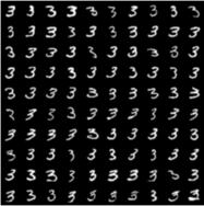
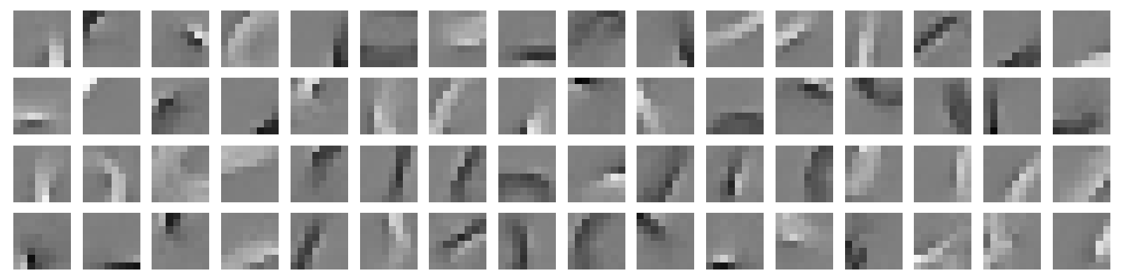
(a)
(a)
(a)
(b)
Figure 2.6: Comparison of learned dictionary atoms for complete (orthogonal) and overcomplete dictionaries, trained to reconstruct 888 by 888 patches taken from MNIST digits. Both dictionaries are trained for 600060006000 epochs on 10410^{4}10 start_POSTSUPERSCRIPT 4 end_POSTSUPERSCRIPT random patches with nontrivial content, and sparse codes are computed with the LASSO objective and λ=0.1\lambda=0.1italic_λ = 0.1 (see (2.3.5)). Colormaps have black for negative values, and white for positive values. Top: An orthogonal dictionary learned with the MSP algorithm (2.2.18) is constrained to have no more than 646464 atoms; the learned atoms roughly correspond to a “spike and slab” dictionary, and achieve relatively poor reconstruction sparsity levels on held-out test data (codes are approximately 171717-sparse on average, with respect to a threshold of 10110^{-1}10 start_POSTSUPERSCRIPT - 1 end_POSTSUPERSCRIPT). Bottom: In contrast, an overcomplete dictionary (here, with 838^{3}8 start_POSTSUPERSCRIPT 3 end_POSTSUPERSCRIPT atoms; we visualize a random subset of 646464) learns semantically-meaningful dictionary atoms corresponding to signed oriented edges, which can be pieced together to create digit patches and achieve superior reconstruction and sparisty levels. Codes are approximately 202020-sparse on average, while being 888 times larger than those of the orthogonal dictionary. To compute the dictionary, we use an optimizer based on proximal alternating linearized minimization on a suitably-regularized version of (2.3.17).
Example 2.1.

Given sampled images of hand-written digits, Figure 2.6(a) shows the result of fitting an orthogonal dictionary to the dataset. In contrast, Figure 2.6(b) shows the result of running an optimization algorithm for learning overcomplete dictionaries (which we will present in detail later in the Chapter) on these samples. Notice that the representations become far sparser and the codebooks far more interpretable—they consist of fundamental primitives for the strokes composing the digits, i.e. oriented edges. \blacksquare

In fact, overcomplete dictionary learning was originally proposed as a biologically plausible algorithm for image representation based on empirical evidence of how early stages of the visual cortex represent visual stimuli [OF96, OF97].

In the remainder of this section, we will overview the conceptual and computational foundations of overcomplete dictionary learning. Supposing that the model (2.3.1) is satisfied with sparse codes 𝒛\bm{z}bold_italic_z, overcomplete dictionary 𝑨\bm{A}bold_italic_A, and sparsity level dditalic_d, and given samples 𝑿=[𝒙1,,𝒙N]\bm{X}=[\bm{x}_{1},\dots,\bm{x}_{N}]bold_italic_X = [ bold_italic_x start_POSTSUBSCRIPT 1 end_POSTSUBSCRIPT , … , bold_italic_x start_POSTSUBSCRIPT italic_N end_POSTSUBSCRIPT ] of 𝒙\bm{x}bold_italic_x, we want to learn an encoder :Dm\mathcal{E}:\mathbb{R}^{D}\to\mathbb{R}^{m}caligraphic_E : blackboard_R start_POSTSUPERSCRIPT italic_D end_POSTSUPERSCRIPT → blackboard_R start_POSTSUPERSCRIPT italic_m end_POSTSUPERSCRIPT mapping each 𝒙\bm{x}bold_italic_x to its sparse code 𝒛\bm{z}bold_italic_z, and a decoder 𝒟(𝒛)=𝑨𝒛\mathcal{D}(\bm{z})=\bm{A}\bm{z}caligraphic_D ( bold_italic_z ) = bold_italic_A bold_italic_z reconstructing each 𝒙\bm{x}bold_italic_x from its sparse code. In diagram form:

𝒙𝒛𝒟=𝑨𝒙^.\bm{x}\xrightarrow{\hskip 11.38109pt\mathcal{E}\hskip 11.38109pt}\bm{z}\xrightarrow{\hskip 5.69054pt\mathcal{D}=\bm{A}\hskip 5.69054pt}\hat{\bm{x}}.bold_italic_x start_ARROW start_OVERACCENT caligraphic_E end_OVERACCENT → end_ARROW bold_italic_z start_ARROW start_OVERACCENT caligraphic_D = bold_italic_A end_OVERACCENT → end_ARROW over^ start_ARG bold_italic_x end_ARG . (2.3.2)

We will start from the construction of the encoder \mathcal{E}caligraphic_E. We will work incrementally: first, given the true dictionary 𝐀\bm{A}bold_italic_A, we will show how the problem of sparse coding gives an elegant, scalable, and provably-correct algorithm for recovering the sparse code 𝒛\bm{z}bold_italic_z of 𝒙\bm{x}bold_italic_x. Although this problem is NP-hard in the worst case, it can be solved efficiently and scalably for dictionaries 𝑨\bm{A}bold_italic_A which are incoherent, i.e. having columns that are not too correlated. The encoder architecture encompassed by this solution will no longer be symmetric: we will see it has the form of a primitive deep network, which depends on the dictionary 𝑨\bm{A}bold_italic_A.

Then we will proceed to the task of learning the decoder 𝒟\mathcal{D}caligraphic_D, or equivalently the overcomplete dictionary 𝑨\bm{A}bold_italic_A. We will derive an algorithm for overcomplete dictionary learning that allows us to simultaneously learn the codebook 𝑨\bm{A}bold_italic_A and the sparse codes 𝒛\bm{z}bold_italic_z, using ideas from sparse coding. Finally, we will discuss a more modern perspective on learnable sparse coding that leads us to a fully asymmetric encoder-decoder structure, as an alternative to (2.3.2). Here, the decoder will correspond to an incremental solution to the sparse dictionary learning problem, and yield a pair of deep network-like encoder decoders for sparse dictionary learning. This structure will foreshadow many developments to come in the remainder of the monograph, as we progress from analytical models to modern neural networks.

2.3.1 Sparse Coding with an Overcomplete Dictionary

In this section, we will consider the data model (2.3.1), which accommodates sparse linear combinations of many motifs, or atoms. Given data {𝒙i}i=1ND\{\bm{x}_{i}\}_{i=1}^{N}\subseteq\mathbb{R}^{D}{ bold_italic_x start_POSTSUBSCRIPT italic_i end_POSTSUBSCRIPT } start_POSTSUBSCRIPT italic_i = 1 end_POSTSUBSCRIPT start_POSTSUPERSCRIPT italic_N end_POSTSUPERSCRIPT ⊆ blackboard_R start_POSTSUPERSCRIPT italic_D end_POSTSUPERSCRIPT satisfying this model, i.e. expressible as

𝒙i=𝑨𝒛i+𝜺i,i[N]\bm{x}_{i}=\bm{A}\bm{z}_{i}+\bm{\varepsilon}_{i},\qquad\forall i\in[N]bold_italic_x start_POSTSUBSCRIPT italic_i end_POSTSUBSCRIPT = bold_italic_A bold_italic_z start_POSTSUBSCRIPT italic_i end_POSTSUBSCRIPT + bold_italic_ε start_POSTSUBSCRIPT italic_i end_POSTSUBSCRIPT , ∀ italic_i ∈ [ italic_N ] (2.3.3)

for some dictionary 𝑨D×m\bm{A}\in\mathbb{R}^{D\times m}bold_italic_A ∈ blackboard_R start_POSTSUPERSCRIPT italic_D × italic_m end_POSTSUPERSCRIPT with mmitalic_m atoms, sparse codes 𝒛i\bm{z}_{i}bold_italic_z start_POSTSUBSCRIPT italic_i end_POSTSUBSCRIPT such that 𝒛i0d\|\bm{z}_{i}\|_{0}\leq d∥ bold_italic_z start_POSTSUBSCRIPT italic_i end_POSTSUBSCRIPT ∥ start_POSTSUBSCRIPT 0 end_POSTSUBSCRIPT ≤ italic_d, and small errors 𝜺i\bm{\varepsilon}_{i}bold_italic_ε start_POSTSUBSCRIPT italic_i end_POSTSUBSCRIPT, the sparse coding problem is to recover the codes 𝒛i\bm{z}_{i}bold_italic_z start_POSTSUBSCRIPT italic_i end_POSTSUBSCRIPT as accurately as possible from the data 𝒙i\bm{x}_{i}bold_italic_x start_POSTSUBSCRIPT italic_i end_POSTSUBSCRIPT, given the dictionary 𝑨\bm{A}bold_italic_A. Efficient algorithms to solve this problem succeed when the dictionary 𝑨\bm{A}bold_italic_A is incoherent in the sense that the inner products 𝒂i𝒂j\bm{a}_{i}^{\top}\bm{a}_{j}bold_italic_a start_POSTSUBSCRIPT italic_i end_POSTSUBSCRIPT start_POSTSUPERSCRIPT ⊤ end_POSTSUPERSCRIPT bold_italic_a start_POSTSUBSCRIPT italic_j end_POSTSUBSCRIPT are uniformly small, hence the atoms are nearly orthogonal.101010As it turns out, in a high-dimensional space, it is rather easy to pack a number of nearly orthogonal vectors that is much larger than the ambient dimension [WM22].

Note that we can collect the 𝒙i\bm{x}_{i}bold_italic_x start_POSTSUBSCRIPT italic_i end_POSTSUBSCRIPT into 𝑿=[𝒙1,,𝒙N]D×N\bm{X}=\begin{bmatrix}\bm{x}_{1},\dots,\bm{x}_{N}\end{bmatrix}\in\mathbb{R}^{D\times N}bold_italic_X = [ start_ARG start_ROW start_CELL bold_italic_x start_POSTSUBSCRIPT 1 end_POSTSUBSCRIPT , … , bold_italic_x start_POSTSUBSCRIPT italic_N end_POSTSUBSCRIPT end_CELL end_ROW end_ARG ] ∈ blackboard_R start_POSTSUPERSCRIPT italic_D × italic_N end_POSTSUPERSCRIPT, collect the 𝒛i\bm{z}_{i}bold_italic_z start_POSTSUBSCRIPT italic_i end_POSTSUBSCRIPT into 𝒁=[𝒛1,,𝒛N]d×N\bm{Z}=\begin{bmatrix}\bm{z}_{1},\dots,\bm{z}_{N}\end{bmatrix}\in\mathbb{R}^{d\times N}bold_italic_Z = [ start_ARG start_ROW start_CELL bold_italic_z start_POSTSUBSCRIPT 1 end_POSTSUBSCRIPT , … , bold_italic_z start_POSTSUBSCRIPT italic_N end_POSTSUBSCRIPT end_CELL end_ROW end_ARG ] ∈ blackboard_R start_POSTSUPERSCRIPT italic_d × italic_N end_POSTSUPERSCRIPT, and collect the 𝜺i\bm{\varepsilon}_{i}bold_italic_ε start_POSTSUBSCRIPT italic_i end_POSTSUBSCRIPT into 𝑬=[𝜺1,,𝜺N]D×N\bm{E}=\begin{bmatrix}\bm{\varepsilon}_{1},\dots,\bm{\varepsilon}_{N}\end{bmatrix}\in\mathbb{R}^{D\times N}bold_italic_E = [ start_ARG start_ROW start_CELL bold_italic_ε start_POSTSUBSCRIPT 1 end_POSTSUBSCRIPT , … , bold_italic_ε start_POSTSUBSCRIPT italic_N end_POSTSUBSCRIPT end_CELL end_ROW end_ARG ] ∈ blackboard_R start_POSTSUPERSCRIPT italic_D × italic_N end_POSTSUPERSCRIPT, to rewrite (2.3.3) as

𝑿=𝑨𝒁+𝑬.\bm{X}=\bm{A}\bm{Z}+\bm{E}.bold_italic_X = bold_italic_A bold_italic_Z + bold_italic_E . (2.3.4)

A natural approach to solving the sparse coding problem is to seek the sparsest signals that are consistent with our observations, and this naturally leads to the following optimization problem:

min𝒁d×N{𝑿𝑨𝒁F2+λ𝒁1},\min_{\bm{Z}\in\mathbb{R}^{d\times N}}\left\{\|\bm{X}-\bm{A}\bm{Z}\|_{F}^{2}+\lambda\|\bm{Z}\|_{1}\right\},roman_min start_POSTSUBSCRIPT bold_italic_Z ∈ blackboard_R start_POSTSUPERSCRIPT italic_d × italic_N end_POSTSUPERSCRIPT end_POSTSUBSCRIPT { ∥ bold_italic_X - bold_italic_A bold_italic_Z ∥ start_POSTSUBSCRIPT italic_F end_POSTSUBSCRIPT start_POSTSUPERSCRIPT 2 end_POSTSUPERSCRIPT + italic_λ ∥ bold_italic_Z ∥ start_POSTSUBSCRIPT 1 end_POSTSUBSCRIPT } , (2.3.5)

where the 1\ell^{1}roman_ℓ start_POSTSUPERSCRIPT 1 end_POSTSUPERSCRIPT norm 𝒁1\|\bm{Z}\|_{1}∥ bold_italic_Z ∥ start_POSTSUBSCRIPT 1 end_POSTSUBSCRIPT, taken elementwise, is known to promote sparsity of the solution [WM22]. This optimization problem is known as the LASSO problem.

However, unlike PCA or the complete dictionary learning problem, there is no clear power iteration-type algorithm to recover 𝒁\bm{Z}^{\star}bold_italic_Z start_POSTSUPERSCRIPT ⋆ end_POSTSUPERSCRIPT. A natural alternative is to consider solving the above optimization problem with gradient descent type algorithms. Let f(𝒁)=𝑿𝑨𝒁22+λ𝒁1f(\bm{Z})=\|\bm{X}-\bm{A}\bm{Z}\|_{2}^{2}+\lambda\|\bm{Z}\|_{1}italic_f ( bold_italic_Z ) = ∥ bold_italic_X - bold_italic_A bold_italic_Z ∥ start_POSTSUBSCRIPT 2 end_POSTSUBSCRIPT start_POSTSUPERSCRIPT 2 end_POSTSUPERSCRIPT + italic_λ ∥ bold_italic_Z ∥ start_POSTSUBSCRIPT 1 end_POSTSUBSCRIPT. Conceptually, we could try to find 𝒁\bm{Z}^{\star}bold_italic_Z start_POSTSUPERSCRIPT ⋆ end_POSTSUPERSCRIPT with the following iterations:

𝒁t+1𝒁t+ηf(𝒁t).\bm{Z}_{t+1}\leftarrow\bm{Z}_{t}+\eta\nabla f(\bm{Z}_{t}).bold_italic_Z start_POSTSUBSCRIPT italic_t + 1 end_POSTSUBSCRIPT ← bold_italic_Z start_POSTSUBSCRIPT italic_t end_POSTSUBSCRIPT + italic_η ∇ italic_f ( bold_italic_Z start_POSTSUBSCRIPT italic_t end_POSTSUBSCRIPT ) . (2.3.6)

However, because the term associated with the 1\ell^{1}roman_ℓ start_POSTSUPERSCRIPT 1 end_POSTSUPERSCRIPT norm 𝒁1\|\bm{Z}\|_{1}∥ bold_italic_Z ∥ start_POSTSUBSCRIPT 1 end_POSTSUBSCRIPT is non-smooth, we cannot just run gradient descent. For this type of function, we need to replace the gradient f(𝒁)\nabla f(\bm{Z})∇ italic_f ( bold_italic_Z ) with something that generalizes the notion of gradient, known as the subgradient f(𝒁)\partial f(\bm{Z})∂ italic_f ( bold_italic_Z ):

𝒁t+1𝒁t+ηf(𝒁t).\bm{Z}_{t+1}\leftarrow\bm{Z}_{t}+\eta\partial f(\bm{Z}_{t}).bold_italic_Z start_POSTSUBSCRIPT italic_t + 1 end_POSTSUBSCRIPT ← bold_italic_Z start_POSTSUBSCRIPT italic_t end_POSTSUBSCRIPT + italic_η ∂ italic_f ( bold_italic_Z start_POSTSUBSCRIPT italic_t end_POSTSUBSCRIPT ) . (2.3.7)

However, it is known that the convergence of subgradient descent is usually very slow. Hence, for this type of optimization problems, it is conventional to adopt a so-called proximal gradient descent-type algorithm. We give a technical overview of this method in Section A.1.3.

Applying proximal gradient to the LASSO objective function (2.3.5) leads to the classic iterative shrinkage-thresholding algorithm (ISTA), which implements the iteration

𝒁1\displaystyle\bm{Z}_{1}bold_italic_Z start_POSTSUBSCRIPT 1 end_POSTSUBSCRIPT \displaystyle\sim 𝒩(𝟎,𝑰),\displaystyle\operatorname{\mathcal{N}}(\bm{0},\bm{I}),caligraphic_N ( bold_0 , bold_italic_I ) , (2.3.8)
𝒁t+1\displaystyle\bm{Z}_{t+1}bold_italic_Z start_POSTSUBSCRIPT italic_t + 1 end_POSTSUBSCRIPT =\displaystyle== Sηλ(𝒁t2η𝑨(𝑨𝒁t𝑿)),t1,\displaystyle S_{\eta\lambda}\left(\bm{Z}_{t}-2\eta\bm{A}^{\top}(\bm{A}\bm{Z}_{t}-\bm{X})\right),\quad\forall t\geq 1,italic_S start_POSTSUBSCRIPT italic_η italic_λ end_POSTSUBSCRIPT ( bold_italic_Z start_POSTSUBSCRIPT italic_t end_POSTSUBSCRIPT - 2 italic_η bold_italic_A start_POSTSUPERSCRIPT ⊤ end_POSTSUPERSCRIPT ( bold_italic_A bold_italic_Z start_POSTSUBSCRIPT italic_t end_POSTSUBSCRIPT - bold_italic_X ) ) , ∀ italic_t ≥ 1 , (2.3.9)

with step size η0\eta\geq 0italic_η ≥ 0, and the soft-thresholding operator SαS_{\alpha}italic_S start_POSTSUBSCRIPT italic_α end_POSTSUBSCRIPT defined on scalars by

Sα(x)\displaystyle S_{\alpha}(x)italic_S start_POSTSUBSCRIPT italic_α end_POSTSUBSCRIPT ( italic_x ) {xα,xα,0,α<x<α,x+α,xα\displaystyle\doteq\begin{cases}x-\alpha,&x\geq\alpha,\\ 0,&-\alpha<x<\alpha,\\ x+\alpha,&x\leq-\alpha\end{cases}≐ { start_ROW start_CELL italic_x - italic_α , end_CELL start_CELL italic_x ≥ italic_α , end_CELL end_ROW start_ROW start_CELL 0 , end_CELL start_CELL - italic_α < italic_x < italic_α , end_CELL end_ROW start_ROW start_CELL italic_x + italic_α , end_CELL start_CELL italic_x ≤ - italic_α end_CELL end_ROW (2.3.10)
=sign(x)max{|x|α,0},\displaystyle=\operatorname{sign}(x)\max\{\lvert x\rvert-\alpha,0\},= roman_sign ( italic_x ) roman_max { | italic_x | - italic_α , 0 } , (2.3.11)

and applied element-wise to the input matrix. As a proximal gradient descent algorithm applied to a convex problem, convergence to a global optimum is assured, and a precise convergence rate can be derived straightforwardly [WM22].

We now take a moment to remark on the functional form of the update operator in (2.3.9). It takes the form

𝒁t+1=nonlinearity(𝒁t+linear(linear(𝒁t)+bias)).\bm{Z}_{t+1}=\texttt{nonlinearity}(\bm{Z}_{t}+\texttt{linear}^{\top}(\texttt{linear}(\bm{Z}_{t})+\texttt{bias})).bold_italic_Z start_POSTSUBSCRIPT italic_t + 1 end_POSTSUBSCRIPT = nonlinearity ( bold_italic_Z start_POSTSUBSCRIPT italic_t end_POSTSUBSCRIPT + linear start_POSTSUPERSCRIPT ⊤ end_POSTSUPERSCRIPT ( linear ( bold_italic_Z start_POSTSUBSCRIPT italic_t end_POSTSUBSCRIPT ) + bias ) ) . (2.3.12)

This functional form is very similar to that of a residual network layer, namely,

𝒁t+1=𝒁t+linear1(nonlinearity(linear2(𝒁t)+bias1)+bias2,\bm{Z}_{t+1}=\bm{Z}_{t}+\texttt{linear}_{1}^{\top}(\texttt{nonlinearity}(\texttt{linear}_{2}(\bm{Z}_{t})+\texttt{bias}_{1})+\texttt{bias}_{2},bold_italic_Z start_POSTSUBSCRIPT italic_t + 1 end_POSTSUBSCRIPT = bold_italic_Z start_POSTSUBSCRIPT italic_t end_POSTSUBSCRIPT + linear start_POSTSUBSCRIPT 1 end_POSTSUBSCRIPT start_POSTSUPERSCRIPT ⊤ end_POSTSUPERSCRIPT ( nonlinearity ( linear start_POSTSUBSCRIPT 2 end_POSTSUBSCRIPT ( bold_italic_Z start_POSTSUBSCRIPT italic_t end_POSTSUBSCRIPT ) + bias start_POSTSUBSCRIPT 1 end_POSTSUBSCRIPT ) + bias start_POSTSUBSCRIPT 2 end_POSTSUBSCRIPT , (2.3.13)

only decoupling the linear maps (i.e., matrix multiplications), adding a bias, and moving the nonlinearity. The nonlinearity in (2.3.9) is notably similar to the commonly-used ReLU activation function xmax{x,0}x\mapsto\max\{x,0\}italic_x ↦ roman_max { italic_x , 0 } in deep learning—in particular, the soft-thresholding operator is like a “signed” ReLU activation, which is also shifted by a bias. The ISTA, then, can be viewed as a forward pass of a primitive (recurrent one-layer) neural network. We argue in Chapter 4 that such operations are essential to deep representation learning.

2.3.2 Overcomplete Dictionary Learning

Recall that we have the data model

𝑿=𝑨𝒁+𝑬,\bm{X}=\bm{A}\bm{Z}+\bm{E},bold_italic_X = bold_italic_A bold_italic_Z + bold_italic_E , (2.3.14)

where 𝒁\bm{Z}bold_italic_Z is sparse, and our goal previously was to estimate 𝒁\bm{Z}bold_italic_Z given knowledge of the data 𝑿\bm{X}bold_italic_X and the dictionary atoms 𝑨\bm{A}bold_italic_A. Now we turn to the more practical and more difficult case where we do not know either 𝑨\bm{A}bold_italic_A or 𝒁\bm{Z}bold_italic_Z and seek to learn them from a large dataset.

A direct generalization of Equation 2.3.5 suggests solving the problem

min𝑨~,𝒁~{𝑿𝑨~𝒁~F2+λ𝒁~1}.\min_{\tilde{\bm{A}},\tilde{\bm{Z}}}\left\{\|\bm{X}-\tilde{\bm{A}}\tilde{\bm{Z}}\|_{F}^{2}+\lambda\|\tilde{\bm{Z}}\|_{1}\right\}.roman_min start_POSTSUBSCRIPT over~ start_ARG bold_italic_A end_ARG , over~ start_ARG bold_italic_Z end_ARG end_POSTSUBSCRIPT { ∥ bold_italic_X - over~ start_ARG bold_italic_A end_ARG over~ start_ARG bold_italic_Z end_ARG ∥ start_POSTSUBSCRIPT italic_F end_POSTSUBSCRIPT start_POSTSUPERSCRIPT 2 end_POSTSUPERSCRIPT + italic_λ ∥ over~ start_ARG bold_italic_Z end_ARG ∥ start_POSTSUBSCRIPT 1 end_POSTSUBSCRIPT } . (2.3.15)

However, the bilinear term in Equation 2.3.15 introduces a scale ambiguity that hinders convergence: given any point (𝑨~,𝒁~)(\tilde{\bm{A}},\tilde{\bm{Z}})( over~ start_ARG bold_italic_A end_ARG , over~ start_ARG bold_italic_Z end_ARG ) and any constant c>0c>0italic_c > 0, the substitution (c1𝑨~,c𝒁~)(c^{-1}\tilde{\bm{A}},c\tilde{\bm{Z}})( italic_c start_POSTSUPERSCRIPT - 1 end_POSTSUPERSCRIPT over~ start_ARG bold_italic_A end_ARG , italic_c over~ start_ARG bold_italic_Z end_ARG ) gives loss value

𝑿𝑨~𝒁~F2+cλ𝒁~1.\|\bm{X}-\tilde{\bm{A}}\tilde{\bm{Z}}\|_{F}^{2}+c\lambda\|\tilde{\bm{Z}}\|_{1}.∥ bold_italic_X - over~ start_ARG bold_italic_A end_ARG over~ start_ARG bold_italic_Z end_ARG ∥ start_POSTSUBSCRIPT italic_F end_POSTSUBSCRIPT start_POSTSUPERSCRIPT 2 end_POSTSUPERSCRIPT + italic_c italic_λ ∥ over~ start_ARG bold_italic_Z end_ARG ∥ start_POSTSUBSCRIPT 1 end_POSTSUBSCRIPT . (2.3.16)

This loss is evidently minimized over ccitalic_c by taking c0c\to 0italic_c → 0, which corresponds to making the rescaled dictionary c1𝑨~c^{-1}\tilde{\bm{A}}italic_c start_POSTSUPERSCRIPT - 1 end_POSTSUPERSCRIPT over~ start_ARG bold_italic_A end_ARG go ‘to infinity’. In particular, the iterates of any optimization algorithm solving (2.3.15) will not converge.

This issue with (2.3.15) is dealt with by adding a constraint on the scale of the columns of the dictionary 𝑨~\tilde{\bm{A}}over~ start_ARG bold_italic_A end_ARG. For example, it is common to assume that each column 𝑨j\bm{A}_{j}bold_italic_A start_POSTSUBSCRIPT italic_j end_POSTSUBSCRIPT of the dictionary 𝑨\bm{A}bold_italic_A in (2.3.14) has bounded 2\ell^{2}roman_ℓ start_POSTSUPERSCRIPT 2 end_POSTSUPERSCRIPT norm—say, without loss of generality, by 111. We then enforce this as a constraint, giving the objective

min𝒁~,𝑨~:𝑨~j21{𝑿𝑨~𝒁~F2+λ𝒁~1}.\min_{\tilde{\bm{Z}},\tilde{\bm{A}}\,:\,\|\tilde{\bm{A}}_{j}\|_{2}\leq 1}\left\{\|\bm{X}-\tilde{\bm{A}}\tilde{\bm{Z}}\|_{F}^{2}+\lambda\|\tilde{\bm{Z}}\|_{1}\right\}.roman_min start_POSTSUBSCRIPT over~ start_ARG bold_italic_Z end_ARG , over~ start_ARG bold_italic_A end_ARG : ∥ over~ start_ARG bold_italic_A end_ARG start_POSTSUBSCRIPT italic_j end_POSTSUBSCRIPT ∥ start_POSTSUBSCRIPT 2 end_POSTSUBSCRIPT ≤ 1 end_POSTSUBSCRIPT { ∥ bold_italic_X - over~ start_ARG bold_italic_A end_ARG over~ start_ARG bold_italic_Z end_ARG ∥ start_POSTSUBSCRIPT italic_F end_POSTSUBSCRIPT start_POSTSUPERSCRIPT 2 end_POSTSUPERSCRIPT + italic_λ ∥ over~ start_ARG bold_italic_Z end_ARG ∥ start_POSTSUBSCRIPT 1 end_POSTSUBSCRIPT } . (2.3.17)

Constrained optimization problems such as (2.3.17) can be solved by a host of sophisticated algorithms [NW06]. However, a simple and scalable one is actually furnished by the same proximal gradient descent algorithm that we used to solve the sparse coding problem in the previous section. We can encode each constraint as additional regularization term, via the characteristic function for the constraint set—details are given in Example A.1. Applying proximal gradient descent to the resulting regularized problem is equivalent to projected gradient descent, in which, at each iteration, the iterates after taking a gradient descent step are projected onto the constraint set.

Remark 2.11 (4\ell^{4}roman_ℓ start_POSTSUPERSCRIPT 4 end_POSTSUPERSCRIPT maximization versus 1\ell^{1}roman_ℓ start_POSTSUPERSCRIPT 1 end_POSTSUPERSCRIPT minimization).

Note that the above problem formulation follows naturally from the LASSO formulation (2.3.5) for sparse coding. We promote the sparsity of the solution via the 1\ell^{1}roman_ℓ start_POSTSUPERSCRIPT 1 end_POSTSUPERSCRIPT norm. Nevertheless, if we are only interested in recovering the over-complete dictionary 𝑨\bm{A}bold_italic_A, the 4\ell^{4}roman_ℓ start_POSTSUPERSCRIPT 4 end_POSTSUPERSCRIPT maximization scheme introduced in Section 2.2.2 also generalizes to the over-complete case, without any significant modification. Interested readers may refer to the work of [QZL+20].

The above problem (2.3.17), which we call overcomplete dictionary learning, is nonconvex as here both 𝑨\bm{A}bold_italic_A and 𝒁\bm{Z}bold_italic_Z are unknown. It cannot be solved easily by the standard convex optimization toolkit. Nevertheless, because it is interesting, simple to state, and practically important, there have been many important works dedicated to different algorithms and theoretical analysis for this problem. Here, for the interest of this manuscript, we present an idiomatic approach to solve this problem which is closer to the spirit of deep learning.

From our experience with the LASSO problem above, it is easy to see that, for the two unknowns 𝑨\bm{A}bold_italic_A and 𝒁\bm{Z}bold_italic_Z, if we fix one and optimize the other, each subproblem is in fact convex and easy to solve. This naturally suggests that we could attempt to solve the above program (2.3.17) by minimizing against 𝒁\bm{Z}bold_italic_Z or 𝑨\bm{A}bold_italic_A alternatively, say using gradient descent. Coupled with a natural choice of initialization, this leads to the following iterative scheme:

𝒁+1=Sηλ(𝒁2η𝑨+(𝑨+𝒁𝑿)),𝒁1=𝟎,[L]\displaystyle\bm{Z}^{\ell+1}=S_{\eta\lambda}\left(\bm{Z}^{\ell}-2\eta\bm{A}_{+}^{\top}(\bm{A}_{+}\bm{Z}^{\ell}-\bm{X})\right),\quad\bm{Z}^{1}=\mathbf{0},\quad\forall\ell\in[L]bold_italic_Z start_POSTSUPERSCRIPT roman_ℓ + 1 end_POSTSUPERSCRIPT = italic_S start_POSTSUBSCRIPT italic_η italic_λ end_POSTSUBSCRIPT ( bold_italic_Z start_POSTSUPERSCRIPT roman_ℓ end_POSTSUPERSCRIPT - 2 italic_η bold_italic_A start_POSTSUBSCRIPT + end_POSTSUBSCRIPT start_POSTSUPERSCRIPT ⊤ end_POSTSUPERSCRIPT ( bold_italic_A start_POSTSUBSCRIPT + end_POSTSUBSCRIPT bold_italic_Z start_POSTSUPERSCRIPT roman_ℓ end_POSTSUPERSCRIPT - bold_italic_X ) ) , bold_italic_Z start_POSTSUPERSCRIPT 1 end_POSTSUPERSCRIPT = bold_0 , ∀ roman_ℓ ∈ [ italic_L ] (2.3.18)
𝒁+=𝒁L,\displaystyle\bm{Z}^{+}=\bm{Z}^{L},bold_italic_Z start_POSTSUPERSCRIPT + end_POSTSUPERSCRIPT = bold_italic_Z start_POSTSUPERSCRIPT italic_L end_POSTSUPERSCRIPT , (2.3.19)
𝑨t+1=proj()j21,j(𝑨t2ν(𝑨t𝒁+𝑿)(𝒁+)),(𝑨1)ji.i.d.𝒩(𝟎,1D𝑰),j[m],t[T],\displaystyle\bm{A}_{t+1}=\operatorname{proj}_{\|(\,\cdot\,)_{j}\|_{2}\leq 1,\,\forall j}\left(\bm{A}_{t}-2\nu(\bm{A}_{t}\bm{Z}^{+}-\bm{X})(\bm{Z}^{+})^{\top}\right),\quad(\bm{A}_{1})_{j}\stackrel{{\scriptstyle\mathrm{i.i.d.}}}{{\sim}}\operatorname{\mathcal{N}}(\bm{0},\tfrac{1}{D}\bm{I}),\enspace\forall j\in[m],\quad\;\;\forall t\in[T],bold_italic_A start_POSTSUBSCRIPT italic_t + 1 end_POSTSUBSCRIPT = roman_proj start_POSTSUBSCRIPT ∥ ( ⋅ ) start_POSTSUBSCRIPT italic_j end_POSTSUBSCRIPT ∥ start_POSTSUBSCRIPT 2 end_POSTSUBSCRIPT ≤ 1 , ∀ italic_j end_POSTSUBSCRIPT ( bold_italic_A start_POSTSUBSCRIPT italic_t end_POSTSUBSCRIPT - 2 italic_ν ( bold_italic_A start_POSTSUBSCRIPT italic_t end_POSTSUBSCRIPT bold_italic_Z start_POSTSUPERSCRIPT + end_POSTSUPERSCRIPT - bold_italic_X ) ( bold_italic_Z start_POSTSUPERSCRIPT + end_POSTSUPERSCRIPT ) start_POSTSUPERSCRIPT ⊤ end_POSTSUPERSCRIPT ) , ( bold_italic_A start_POSTSUBSCRIPT 1 end_POSTSUBSCRIPT ) start_POSTSUBSCRIPT italic_j end_POSTSUBSCRIPT start_RELOP SUPERSCRIPTOP start_ARG ∼ end_ARG start_ARG roman_i . roman_i . roman_d . end_ARG end_RELOP caligraphic_N ( bold_0 , divide start_ARG 1 end_ARG start_ARG italic_D end_ARG bold_italic_I ) , ∀ italic_j ∈ [ italic_m ] , ∀ italic_t ∈ [ italic_T ] , (2.3.20)
𝑨+=𝑨T,\displaystyle\bm{A}_{+}=\bm{A}_{T},bold_italic_A start_POSTSUBSCRIPT + end_POSTSUBSCRIPT = bold_italic_A start_POSTSUBSCRIPT italic_T end_POSTSUBSCRIPT , (2.3.21)

where the projection operation in the update for 𝑨\bm{A}bold_italic_A ensures each column has at most unit 2\ell^{2}roman_ℓ start_POSTSUPERSCRIPT 2 end_POSTSUPERSCRIPT norm, via 𝑨j𝑨j/max{𝑨j2,1}\bm{A}_{j}\mapsto\bm{A}_{j}/\max\{\|\bm{A}_{j}\|_{2},1\}bold_italic_A start_POSTSUBSCRIPT italic_j end_POSTSUBSCRIPT ↦ bold_italic_A start_POSTSUBSCRIPT italic_j end_POSTSUBSCRIPT / roman_max { ∥ bold_italic_A start_POSTSUBSCRIPT italic_j end_POSTSUBSCRIPT ∥ start_POSTSUBSCRIPT 2 end_POSTSUBSCRIPT , 1 }, and where 𝑨+\bm{A}_{+}bold_italic_A start_POSTSUBSCRIPT + end_POSTSUBSCRIPT is initialized with each column i.i.d. 𝒩(𝟎,1D𝑰)\mathcal{N}(\mathbf{0},\tfrac{1}{D}\bm{I})caligraphic_N ( bold_0 , divide start_ARG 1 end_ARG start_ARG italic_D end_ARG bold_italic_I ). The above consists of one ‘block’ of alternating minimization, and we repeatedly perform such blocks, each with independent initializations, until convergence. Above, we have used two separate indices {t}\{t\}{ italic_t } and {}\{\ell\}{ roman_ℓ } to indicate the iterations. As we will see later, this allows us to interpret the two updates separately in the context of deep learning.

Despite the dictionary learning problem being a nonconvex problem, it has been shown that alternating minimization type algorithms indeed converge to the correct solution, at least locally. See, for example, [AAJ+16]. As a practical demonstration, the above algorithm (with L=T=1L=T=1italic_L = italic_T = 1) was used to generate the results for overcomplete dictionary learning in Figure 2.6.

2.3.3 Learned Deep Sparse Coding

The main insight from the alternating minimization algorithm for overcomplete dictionary learning in the previous section (Equations 2.3.18 and 2.3.20) is to notice that when we fix 𝐀\bm{A}bold_italic_A, the ISTA update for 𝐙\bm{Z}^{\ell}bold_italic_Z start_POSTSUPERSCRIPT roman_ℓ end_POSTSUPERSCRIPT (2.3.18) looks like the forward pass of a deep neural network with weights given by 𝐀\bm{A}bold_italic_A (and 𝐀\bm{A}^{\top}bold_italic_A start_POSTSUPERSCRIPT ⊤ end_POSTSUPERSCRIPT). But in general, we do not know the true 𝑨\bm{A}bold_italic_A, and the current estimate 𝑨+\bm{A}_{+}bold_italic_A start_POSTSUBSCRIPT + end_POSTSUBSCRIPT could be erroneous. Hence it needs to be further updated using (2.3.20) based on the residual of using the current estimate of the sparse codes 𝒁+\bm{Z}^{+}bold_italic_Z start_POSTSUPERSCRIPT + end_POSTSUPERSCRIPT to reconstruct 𝑿\bm{X}bold_italic_X. The alternating minimization algorithm iterates these two procedures until convergence. But we can instead extrapolate, and design other learning procedures by combining these insights with techniques from deep learning. This leads to more interpretable network architectures, which will be a recurring theme throughout this manuscript.

Learned ISTA.

The above deep-network interpretation of the alternating minimization is more conceptual than practical, as the process could be rather inefficient and take many layers or iterations to converge. But this is mainly because we try to infer both 𝒁\bm{Z}bold_italic_Z and 𝑨\bm{A}bold_italic_A from 𝑿\bm{X}bold_italic_X. The problem can be significantly simplified and the above iterations can be made much more efficient in the supervised setting, where we have a dataset of input and output pairs (𝑿,𝒁)(\bm{X},\bm{Z})( bold_italic_X , bold_italic_Z ) distributed according to (2.3.14) and we only seek to learn 𝑨\bm{A}^{\ell}bold_italic_A start_POSTSUPERSCRIPT roman_ℓ end_POSTSUPERSCRIPT for the layerwise learnable sparse coding iterations (2.3.29):

𝒁+1=Sηλ(𝒁2η(𝑨)(𝑨𝒁𝑿)),[L].\displaystyle\bm{Z}^{\ell+1}=S_{\eta\lambda}\left(\bm{Z}^{\ell}-2\eta(\bm{A}^{\ell})^{\top}(\bm{A}^{\ell}\bm{Z}^{\ell}-\bm{X})\right),\quad\forall\ell\in[L].bold_italic_Z start_POSTSUPERSCRIPT roman_ℓ + 1 end_POSTSUPERSCRIPT = italic_S start_POSTSUBSCRIPT italic_η italic_λ end_POSTSUBSCRIPT ( bold_italic_Z start_POSTSUPERSCRIPT roman_ℓ end_POSTSUPERSCRIPT - 2 italic_η ( bold_italic_A start_POSTSUPERSCRIPT roman_ℓ end_POSTSUPERSCRIPT ) start_POSTSUPERSCRIPT ⊤ end_POSTSUPERSCRIPT ( bold_italic_A start_POSTSUPERSCRIPT roman_ℓ end_POSTSUPERSCRIPT bold_italic_Z start_POSTSUPERSCRIPT roman_ℓ end_POSTSUPERSCRIPT - bold_italic_X ) ) , ∀ roman_ℓ ∈ [ italic_L ] . (2.3.22)

If we denote the operator for each iteration as 𝒁+1=f(𝑨,𝒁)\bm{Z}^{\ell+1}=f(\bm{A}^{\ell},\bm{Z}^{\ell})bold_italic_Z start_POSTSUPERSCRIPT roman_ℓ + 1 end_POSTSUPERSCRIPT = italic_f ( bold_italic_A start_POSTSUPERSCRIPT roman_ℓ end_POSTSUPERSCRIPT , bold_italic_Z start_POSTSUPERSCRIPT roman_ℓ end_POSTSUPERSCRIPT ), the above iteration can be illustrated in terms of a diagram:

𝑿,𝒁1f(𝑨1,)𝒁2f(𝑨2,)𝒁3f(𝑨3,)𝒁Lf(𝑨L,)𝒁L+1𝒁.\bm{X},\bm{Z}^{1}\xrightarrow{\hskip 2.84526ptf(\bm{A}^{1},\,\cdot\,)\hskip 2.84526pt}\bm{Z}^{2}\xrightarrow{\hskip 2.84526ptf(\bm{A}^{2},\,\cdot\,)\hskip 2.84526pt}\bm{Z}^{3}\xrightarrow{\hskip 2.84526ptf(\bm{A}^{3},\,\cdot\,)\hskip 2.84526pt}\cdots\bm{Z}^{L}\xrightarrow{\hskip 2.84526ptf(\bm{A}^{L},\,\cdot\,)\hskip 2.84526pt}\bm{Z}^{L+1}\approx\bm{Z}.bold_italic_X , bold_italic_Z start_POSTSUPERSCRIPT 1 end_POSTSUPERSCRIPT start_ARROW start_OVERACCENT italic_f ( bold_italic_A start_POSTSUPERSCRIPT 1 end_POSTSUPERSCRIPT , ⋅ ) end_OVERACCENT → end_ARROW bold_italic_Z start_POSTSUPERSCRIPT 2 end_POSTSUPERSCRIPT start_ARROW start_OVERACCENT italic_f ( bold_italic_A start_POSTSUPERSCRIPT 2 end_POSTSUPERSCRIPT , ⋅ ) end_OVERACCENT → end_ARROW bold_italic_Z start_POSTSUPERSCRIPT 3 end_POSTSUPERSCRIPT start_ARROW start_OVERACCENT italic_f ( bold_italic_A start_POSTSUPERSCRIPT 3 end_POSTSUPERSCRIPT , ⋅ ) end_OVERACCENT → end_ARROW ⋯ bold_italic_Z start_POSTSUPERSCRIPT italic_L end_POSTSUPERSCRIPT start_ARROW start_OVERACCENT italic_f ( bold_italic_A start_POSTSUPERSCRIPT italic_L end_POSTSUPERSCRIPT , ⋅ ) end_OVERACCENT → end_ARROW bold_italic_Z start_POSTSUPERSCRIPT italic_L + 1 end_POSTSUPERSCRIPT ≈ bold_italic_Z .

Thus, given the sequential architecture, to learn the operator 𝑨\bm{A}^{\ell}bold_italic_A start_POSTSUPERSCRIPT roman_ℓ end_POSTSUPERSCRIPT at each layer, it is completely natural to learn it, say via back propagation (BP),111111See Section A.2 for a brief description of BP. by minimizing the error between the final code 𝒁L\bm{Z}^{L}bold_italic_Z start_POSTSUPERSCRIPT italic_L end_POSTSUPERSCRIPT and the ground truth 𝒁\bm{Z}bold_italic_Z:

min{𝑨}𝒁L(𝑨1,,𝑨L)𝒁22.\min_{\{\bm{A}^{\ell}\}}\big{\|}\bm{Z}^{L}(\bm{A}^{1},\ldots,\bm{A}^{L})-\bm{Z}\big{\|}_{2}^{2}.roman_min start_POSTSUBSCRIPT { bold_italic_A start_POSTSUPERSCRIPT roman_ℓ end_POSTSUPERSCRIPT } end_POSTSUBSCRIPT ∥ bold_italic_Z start_POSTSUPERSCRIPT italic_L end_POSTSUPERSCRIPT ( bold_italic_A start_POSTSUPERSCRIPT 1 end_POSTSUPERSCRIPT , … , bold_italic_A start_POSTSUPERSCRIPT italic_L end_POSTSUPERSCRIPT ) - bold_italic_Z ∥ start_POSTSUBSCRIPT 2 end_POSTSUBSCRIPT start_POSTSUPERSCRIPT 2 end_POSTSUPERSCRIPT . (2.3.23)

This is the basis of the Learned ISTA (LISTA) algorithm [GL10], which can be viewed as the learning algorithm for a deep neural network, which tries to emulate the sparse encoding process from 𝑿\bm{X}bold_italic_X to 𝒁\bm{Z}bold_italic_Z. In particular, it can be viewed as a simple representation learning algorithm. In fact, this same methodology can be used as a basis to understand the representations computed in more powerful network architectures, such as transformers. We develop these implications in detail in Chapter 4.

Sparse Autoencoders.

The original motivation for overcomplete dictionary learning was to provide a simple generative model for high-dimensional data. We have seen with LISTA that, in addition, iterative algorithms for learning sparsely-used overcomplete dictionaries provide an interpretation for ReLU-like deep networks, which we will generalize in later chapters to more complex data distributions than (2.3.14). But it is also worth noting that even in the modern era of large models, the data generating model (2.3.14) provides a useful practical basis for interpreting features in pretrained large-scale deep networks, such as transformers, following the hypothesis that the (non-interpretable, a priori) features in these networks consist of sparse “superpositions” of underlying features, which are themselves interpretable [EHO+22a]. These unsupervised learning paradigms are generally more data friendly than LISTA, as well, which requires large amounts of labeled (𝑿,𝒁)(\bm{X},\bm{Z})( bold_italic_X , bold_italic_Z ) pairs for supervised training.

We can use our development of the LISTA algorithm above to understand common practices in this field of research. In the most straightforward instantiation (see [HCS+24, GTT+25]), a large number of features from a pretrained deep network hhitalic_h are collected from different inputs 𝒙i\bm{x}_{i}bold_italic_x start_POSTSUBSCRIPT italic_i end_POSTSUBSCRIPT, which themselves are chosen based on a desired interpretation task.121212For example, the inputs 𝒙i\bm{x}_{i}bold_italic_x start_POSTSUBSCRIPT italic_i end_POSTSUBSCRIPT could correspond to texts containing samples of computer code in different programming languages, with our task being to try to identify interpretable features in a transformer feature map hhitalic_h corresponding to different salient aspects of the input, such as the specific programming language (distinct across input “classes”) or the need to insert a matching parenthesis at the current position (common across input “classes”). We discuss the use of deep networks, and in particular transformers, for text representation learning in greater detail in Chapter 7. For simplicity, we will use hhitalic_h to denote the pre-selected feature map in question, with DDitalic_D-dimensional features; given NNitalic_N sample inputs, let 𝑯D×N\bm{H}\in\mathbb{R}^{D\times N}bold_italic_H ∈ blackboard_R start_POSTSUPERSCRIPT italic_D × italic_N end_POSTSUPERSCRIPT denote the full matrix of features of hhitalic_h. Then a so-called sparse autoencoder f:Ddf:\mathbb{R}^{D}\to\mathbb{R}^{d}italic_f : blackboard_R start_POSTSUPERSCRIPT italic_D end_POSTSUPERSCRIPT → blackboard_R start_POSTSUPERSCRIPT italic_d end_POSTSUPERSCRIPT, with decoder g:dDg:\mathbb{R}^{d}\to\mathbb{R}^{D}italic_g : blackboard_R start_POSTSUPERSCRIPT italic_d end_POSTSUPERSCRIPT → blackboard_R start_POSTSUPERSCRIPT italic_D end_POSTSUPERSCRIPT, is trained via the LASSO loss (2.3.5):

minf,g𝑯g(f(𝑯)))F2+λf(𝑯)1,\min_{f,g}\|\bm{H}-g(f(\bm{H})))\|_{F}^{2}+\lambda\|f(\bm{H})\|_{1},roman_min start_POSTSUBSCRIPT italic_f , italic_g end_POSTSUBSCRIPT ∥ bold_italic_H - italic_g ( italic_f ( bold_italic_H ) ) ) ∥ start_POSTSUBSCRIPT italic_F end_POSTSUBSCRIPT start_POSTSUPERSCRIPT 2 end_POSTSUPERSCRIPT + italic_λ ∥ italic_f ( bold_italic_H ) ∥ start_POSTSUBSCRIPT 1 end_POSTSUBSCRIPT , (2.3.24)

where the sparse autoencoder ffitalic_f takes the form of a one-layer neural network, i.e. f(𝒉i)=σ(𝑾enc(𝒉i𝒃)+𝒃enc)f(\bm{h}_{i})=\sigma(\bm{W}_{\mathrm{enc}}(\bm{h}_{i}-\bm{b})+\bm{b}_{\mathrm{enc}})italic_f ( bold_italic_h start_POSTSUBSCRIPT italic_i end_POSTSUBSCRIPT ) = italic_σ ( bold_italic_W start_POSTSUBSCRIPT roman_enc end_POSTSUBSCRIPT ( bold_italic_h start_POSTSUBSCRIPT italic_i end_POSTSUBSCRIPT - bold_italic_b ) + bold_italic_b start_POSTSUBSCRIPT roman_enc end_POSTSUBSCRIPT ), where σ(x)=max{x,0}\sigma(x)=\max\{x,0\}italic_σ ( italic_x ) = roman_max { italic_x , 0 } is the ReLU activation function, and the decoder ggitalic_g is linear, so that g(𝒛i)=𝑾dec𝒛+𝒃g(\bm{z}_{i})=\bm{W}_{\mathrm{dec}}\bm{z}+\bm{b}italic_g ( bold_italic_z start_POSTSUBSCRIPT italic_i end_POSTSUBSCRIPT ) = bold_italic_W start_POSTSUBSCRIPT roman_dec end_POSTSUBSCRIPT bold_italic_z + bold_italic_b.

The parameterization and training procedure (2.3.24) may initially seem to be an arbitrary application of deep learning to the sparse coding problem, but it is actually highly aligned with the algorithms we have studied above for layerwise sparse coding with a learned dictionary. In particular, recall the LISTA architecture 𝒁L=f(𝑨L,f(𝑨L1,,f(𝑨1,𝑿)))\bm{Z}^{L}=f(\bm{A}^{L},f(\bm{A}^{L-1},\cdots,f(\bm{A}^{1},\bm{X})\cdots))bold_italic_Z start_POSTSUPERSCRIPT italic_L end_POSTSUPERSCRIPT = italic_f ( bold_italic_A start_POSTSUPERSCRIPT italic_L end_POSTSUPERSCRIPT , italic_f ( bold_italic_A start_POSTSUPERSCRIPT italic_L - 1 end_POSTSUPERSCRIPT , ⋯ , italic_f ( bold_italic_A start_POSTSUPERSCRIPT 1 end_POSTSUPERSCRIPT , bold_italic_X ) ⋯ ) ). In the special case L=2L=2italic_L = 2, we have

𝒁2=f(𝑨1,𝑿)=Sηλ(𝒁12η(𝑨1)(𝑨1𝒁1𝑿)).\bm{Z}^{2}=f(\bm{A}^{1},\bm{X})=S_{\eta\lambda}\left(\bm{Z}^{1}-2\eta(\bm{A}^{1})^{\top}(\bm{A}^{1}\bm{Z}^{1}-\bm{X})\right).bold_italic_Z start_POSTSUPERSCRIPT 2 end_POSTSUPERSCRIPT = italic_f ( bold_italic_A start_POSTSUPERSCRIPT 1 end_POSTSUPERSCRIPT , bold_italic_X ) = italic_S start_POSTSUBSCRIPT italic_η italic_λ end_POSTSUBSCRIPT ( bold_italic_Z start_POSTSUPERSCRIPT 1 end_POSTSUPERSCRIPT - 2 italic_η ( bold_italic_A start_POSTSUPERSCRIPT 1 end_POSTSUPERSCRIPT ) start_POSTSUPERSCRIPT ⊤ end_POSTSUPERSCRIPT ( bold_italic_A start_POSTSUPERSCRIPT 1 end_POSTSUPERSCRIPT bold_italic_Z start_POSTSUPERSCRIPT 1 end_POSTSUPERSCRIPT - bold_italic_X ) ) . (2.3.25)

Let us assume that the sparse codes 𝒁\bm{Z}bold_italic_Z in question are nonnegative, i.e., that 𝒁𝟎\bm{Z}\geq\mathbf{0}bold_italic_Z ≥ bold_0.131313In the data generating model (2.3.14), an arbitrary dictionary-and-sparse-code pair (𝑨,𝒁)(\bm{A},\bm{Z})( bold_italic_A , bold_italic_Z ) can be replaced by one in which 𝒁𝟎\bm{Z}\geq\mathbf{0}bold_italic_Z ≥ bold_0 simply by doubling the number of columns in 𝑨\bm{A}bold_italic_A, so from a modeling perspective, this is a very mild assumption. Then (see Example A.3), we can consider an equivalent LISTA architecture obtained from the sparse coding objective with an additional nonnegativity constraint on 𝒁\bm{Z}bold_italic_Z as

𝒁2=f(𝑨1,𝑿)=max{𝒁12η(𝑨1)(𝑨1𝒁1𝑿)λη𝟏,0},\bm{Z}^{2}=f(\bm{A}^{1},\bm{X})=\max\left\{\bm{Z}^{1}-2\eta(\bm{A}^{1})^{\top}(\bm{A}^{1}\bm{Z}^{1}-\bm{X})-\lambda\eta\mathbf{1},0\right\},bold_italic_Z start_POSTSUPERSCRIPT 2 end_POSTSUPERSCRIPT = italic_f ( bold_italic_A start_POSTSUPERSCRIPT 1 end_POSTSUPERSCRIPT , bold_italic_X ) = roman_max { bold_italic_Z start_POSTSUPERSCRIPT 1 end_POSTSUPERSCRIPT - 2 italic_η ( bold_italic_A start_POSTSUPERSCRIPT 1 end_POSTSUPERSCRIPT ) start_POSTSUPERSCRIPT ⊤ end_POSTSUPERSCRIPT ( bold_italic_A start_POSTSUPERSCRIPT 1 end_POSTSUPERSCRIPT bold_italic_Z start_POSTSUPERSCRIPT 1 end_POSTSUPERSCRIPT - bold_italic_X ) - italic_λ italic_η bold_1 , 0 } , (2.3.26)

and after some algebra, express this as

𝒁2=f(𝑨1,𝑿)=max{2η(𝑨1)+(𝒁12η(𝑨1)𝑨1𝒁1λη𝟏),0}.\bm{Z}^{2}=f(\bm{A}^{1},\bm{X})=\max\left\{2\eta(\bm{A}^{1})^{\top}+\left(\bm{Z}^{1}-2\eta(\bm{A}^{1})^{\top}\bm{A}^{1}\bm{Z}^{1}-\lambda\eta\mathbf{1}\right),0\right\}.bold_italic_Z start_POSTSUPERSCRIPT 2 end_POSTSUPERSCRIPT = italic_f ( bold_italic_A start_POSTSUPERSCRIPT 1 end_POSTSUPERSCRIPT , bold_italic_X ) = roman_max { 2 italic_η ( bold_italic_A start_POSTSUPERSCRIPT 1 end_POSTSUPERSCRIPT ) start_POSTSUPERSCRIPT ⊤ end_POSTSUPERSCRIPT + ( bold_italic_Z start_POSTSUPERSCRIPT 1 end_POSTSUPERSCRIPT - 2 italic_η ( bold_italic_A start_POSTSUPERSCRIPT 1 end_POSTSUPERSCRIPT ) start_POSTSUPERSCRIPT ⊤ end_POSTSUPERSCRIPT bold_italic_A start_POSTSUPERSCRIPT 1 end_POSTSUPERSCRIPT bold_italic_Z start_POSTSUPERSCRIPT 1 end_POSTSUPERSCRIPT - italic_λ italic_η bold_1 ) , 0 } . (2.3.27)

Given the ability to change the sparse code initialization 𝒁1\bm{Z}^{1}bold_italic_Z start_POSTSUPERSCRIPT 1 end_POSTSUPERSCRIPT as a learnable parameter (which, in the current framework, must have all columns equal to the same learnable vector), this has the form of a ReLU neural network with learnable bias—identical to the sparse autoencoder ffitalic_f! Moreover, to decode the learned sparse codes 𝒁2\bm{Z}^{2}bold_italic_Z start_POSTSUPERSCRIPT 2 end_POSTSUPERSCRIPT, it is natural to apply the learned dictionary 𝒁2𝑨1𝒁2\bm{Z}^{2}\mapsto\bm{A}^{1}\bm{Z}^{2}bold_italic_Z start_POSTSUPERSCRIPT 2 end_POSTSUPERSCRIPT ↦ bold_italic_A start_POSTSUPERSCRIPT 1 end_POSTSUPERSCRIPT bold_italic_Z start_POSTSUPERSCRIPT 2 end_POSTSUPERSCRIPT. Then the only difference between this and the SAE decoder ggitalic_g is the additional bias 𝒃\bm{b}bold_italic_b, which can technically be absorbed into 𝑯\bm{H}bold_italic_H and ffitalic_f in the training objective (2.3.24).

Thus, the SAE parameterization and training procedure coincides with LISTA training with L=1L=1italic_L = 1, and a modified training objective—using the LASSO objective (2.3.5), which remains unsupervised, instead of the supervised reconstruction loss (2.3.23) used in vanilla LISTA. In particular, we can understand the SAE architecture in terms of our interpretation of the LISTA architecture in terms of layerwise sparse coding in (2.3.29). This connection is suggestive of a host of new design strategies for improving practical interpretability methodology, many of which remain tantalizingly unexplored. We begin to lay out some connections to broader autoencoding methodology in Chapter 5.

Layerwise learned sparse coding?

In the supervised setting, LISTA provides a deep neural network analogue of the sparse coding iteration, with layerwise-learned dictionaries, inspired by alternating minimization; even in the unsupervised setting, the same methodology can be applied to learning, as with sparse autoencoders. But the connection between low-dimensional-structure-seeking optimization algorithms and deep network architectures goes much deeper than this, and suggests an array of scalable and natural neural learning architectures which may even be usable without backpropagation.

As a simple illustration, we return the alternating minimization iterations (2.3.18) and (2.3.20). This scheme randomly re-initializes the dictionary 𝑨1\bm{A}_{1}bold_italic_A start_POSTSUBSCRIPT 1 end_POSTSUBSCRIPT on every such update. An improvement uses instead warm starting, where the residual is generated using the previous estimate 𝑨+\bm{A}_{+}bold_italic_A start_POSTSUBSCRIPT + end_POSTSUBSCRIPT for the dictionary. If we then view each ISTA update (2.3.18) as a layer and allow the associated dictionary, now coupled with the sparse code updates as 𝑨\bm{A}_{\ell}bold_italic_A start_POSTSUBSCRIPT roman_ℓ end_POSTSUBSCRIPT, to update in time, this leads to a “layerwise-learnable” sparse coding scheme:

𝒁1=𝟎,(𝑨1)ji.i.d.𝒩(𝟎,1D𝑰),j[m],\displaystyle\bm{Z}^{1}=\mathbf{0},\quad(\bm{A}_{1})_{j}\stackrel{{\scriptstyle\mathrm{i.i.d.}}}{{\sim}}\operatorname{\mathcal{N}}(\bm{0},\tfrac{1}{D}\bm{I}),\enspace\forall j\in[m],bold_italic_Z start_POSTSUPERSCRIPT 1 end_POSTSUPERSCRIPT = bold_0 , ( bold_italic_A start_POSTSUBSCRIPT 1 end_POSTSUBSCRIPT ) start_POSTSUBSCRIPT italic_j end_POSTSUBSCRIPT start_RELOP SUPERSCRIPTOP start_ARG ∼ end_ARG start_ARG roman_i . roman_i . roman_d . end_ARG end_RELOP caligraphic_N ( bold_0 , divide start_ARG 1 end_ARG start_ARG italic_D end_ARG bold_italic_I ) , ∀ italic_j ∈ [ italic_m ] , (2.3.28)
𝒁+1=Sηλ(𝒁2η(𝑨)(𝑨𝒁𝑿)),\displaystyle\bm{Z}^{\ell+1}=S_{\eta\lambda}\left(\bm{Z}^{\ell}-2\eta(\bm{A}_{\ell})^{\top}(\bm{A}_{\ell}\bm{Z}^{\ell}-\bm{X})\right),bold_italic_Z start_POSTSUPERSCRIPT roman_ℓ + 1 end_POSTSUPERSCRIPT = italic_S start_POSTSUBSCRIPT italic_η italic_λ end_POSTSUBSCRIPT ( bold_italic_Z start_POSTSUPERSCRIPT roman_ℓ end_POSTSUPERSCRIPT - 2 italic_η ( bold_italic_A start_POSTSUBSCRIPT roman_ℓ end_POSTSUBSCRIPT ) start_POSTSUPERSCRIPT ⊤ end_POSTSUPERSCRIPT ( bold_italic_A start_POSTSUBSCRIPT roman_ℓ end_POSTSUBSCRIPT bold_italic_Z start_POSTSUPERSCRIPT roman_ℓ end_POSTSUPERSCRIPT - bold_italic_X ) ) , (2.3.29)
𝑨+1=𝑨2ν(𝑨𝒁+1𝑿)(𝒁+1).\displaystyle\bm{A}_{\ell+1}=\bm{A}_{\ell}-2\nu(\bm{A}_{\ell}\bm{Z}^{\ell+1}-\bm{X})(\bm{Z}^{\ell+1})^{\top}.bold_italic_A start_POSTSUBSCRIPT roman_ℓ + 1 end_POSTSUBSCRIPT = bold_italic_A start_POSTSUBSCRIPT roman_ℓ end_POSTSUBSCRIPT - 2 italic_ν ( bold_italic_A start_POSTSUBSCRIPT roman_ℓ end_POSTSUBSCRIPT bold_italic_Z start_POSTSUPERSCRIPT roman_ℓ + 1 end_POSTSUPERSCRIPT - bold_italic_X ) ( bold_italic_Z start_POSTSUPERSCRIPT roman_ℓ + 1 end_POSTSUPERSCRIPT ) start_POSTSUPERSCRIPT ⊤ end_POSTSUPERSCRIPT . (2.3.30)

Note that this iteration corresponds to a relabeling of (2.3.18) and (2.3.20) for T=L=1T=L=1italic_T = italic_L = 1, over infinitely many blocks. Each of the ‘inner’ steps updating 𝒁\bm{Z}bold_italic_Z can be considered as a one-layer forward pass, while each of the ‘outer’ steps updating 𝑨\bm{A}bold_italic_A can be considered as a one-layer backward pass, of a primitive deep neural network. In particular, this algorithm is the simplest case in which a clear divide between forward optimization and backward learning manifests. This divide is still observed in current neural networks and autoencoders—we will have much more to say about it in Chapter 4 and in Chapter 5.

Notice that the above layer-wise scheme also suggests a plausible alternative to the current end-to-end optimization strategy that primarily relies on back propagation (BP) detailed in Section A.2.3. Freeing training large networks from BP would be one of the biggest challenges and opportunities in the future, as we will discuss more at the end of the book in Chapter 8.

2.4 Summary and Notes

The idealistic models we have presented in this chapter—PCA, ICA, and dictionary learning—were developed over the course of the twentieth century. Many books have been written solely about each method, so we will only attempt here to give a broad overview of the key works and history.

Jolliffe [Jol86] attributes principal component analysis to Pearson [Pea01], and independently Hotelling [Hot33]. In mathematics, the main result on the related problem of low-rank approximation in unitarily invariant norms is attributed to Eckart and Young [EY36], and to Mirsky for full generality [Mir60]. PCA continues to play an important role in research as perhaps the simplest model problem for unsupervised representation learning: as early as the 1980s, works such as [Oja82] and [BH89] used the problem to understand learning in primitive neural networks, and more recently, it has served as a tool for understanding more complex representation learning frameworks, such as diffusion models [WZZ+24].

Independent component analysis was proposed by [BJC85] and pioneered by Aapo Hyvärinen in the 1990s and early 2000s in a series of influential works: see [HO00a] for a summary. As a simple model for structure that arises in practical data, it initially saw significant use in applications such as blind source separation, where each independent component ziz_{i}italic_z start_POSTSUBSCRIPT italic_i end_POSTSUBSCRIPT represents an independent source (such as sound associated to a distinct instrument in a musical recording) that is superimposed to produce the observation 𝒙=𝑼𝒛\bm{x}=\bm{U}\bm{z}bold_italic_x = bold_italic_U bold_italic_z.

The problem of dictionary learning can, in the complete or orthogonal case, be seen as one of the foundational problems of twentieth-century signal processing, particularly in linear systems theory, where the Fourier basis plays the key role; from the 1980s onward, the field of computational harmonic analysis crystallized around the study of alternate such dictionaries for classes of signals in which optimal approximation could only be realized in a basis other than Fourier (e.g., wavelets) [DVD+98]. However, the importance of the case of redundant bases, or overcomplete dictionaries, was only highlighted following the pioneering work of Olshausen and Field [OF96, OF97]. Early subsequent work established the conceptual and algorithmic foundations for learning sparsely-used overcomplete dictionaries, often aimed at representing natural images [Don01, DM03, EA06, MK07, AEB06, MBP14, GJB15]. Later, a significant amount of theoretical interest in the problem, as an important and nontrivial model problem for unsupervised representation learning, led to its study by the signal processing, theoretical machine learning, and theoretical computer science communities, in particular focused on conditions under which the problem could be provably and efficiently solved. A non-exhaustive list of notable works in this line include those of [SWW12] and [SQW17] on the complete case; [AGM+15]; [BKS15]; and [QZL+20]. Many deep theoretical questions about this simple-to-state problem remain open, perhaps in part due to a tension with the problem’s worst-case NP-hardness (e.g., see [Til15]).

Table 2.1: Summary of (generalized) power methods presented in the Chapter
Problem Algorithm Iteration Type of Structure Enforced
PCA Power Method 𝒖t=𝑿𝑿𝒖t𝑿𝑿𝒖t2\bm{u}_{t}=\frac{\bm{X}\bm{X}^{\top}\bm{u}_{t}}{\|\bm{X}\bm{X}^{\top}\bm{u}_{t}\|_{2}}bold_italic_u start_POSTSUBSCRIPT italic_t end_POSTSUBSCRIPT = divide start_ARG bold_italic_X bold_italic_X start_POSTSUPERSCRIPT ⊤ end_POSTSUPERSCRIPT bold_italic_u start_POSTSUBSCRIPT italic_t end_POSTSUBSCRIPT end_ARG start_ARG ∥ bold_italic_X bold_italic_X start_POSTSUPERSCRIPT ⊤ end_POSTSUPERSCRIPT bold_italic_u start_POSTSUBSCRIPT italic_t end_POSTSUBSCRIPT ∥ start_POSTSUBSCRIPT 2 end_POSTSUBSCRIPT end_ARG 111-dim. subspace (unit vector)
ICA FastICA 𝒖t+1=1N𝑿(𝑿𝒖t)33𝒖t1N𝑿(𝑿𝒖t)33𝒖t2\bm{u}_{t+1}=\frac{\tfrac{1}{N}\bm{X}(\bm{X}^{\top}\bm{u}_{t})^{\mathbin{\mathchoice{\raisebox{1.3pt}{$\displaystyle\mathchoice{\scalebox{0.8}{$\displaystyle\odot$}}{\scalebox{0.8}{$\textstyle\odot$}}{\scalebox{0.8}{$\scriptstyle\odot$}}{\scalebox{0.8}{$\scriptscriptstyle\odot$}}$}}{\raisebox{1.3pt}{$\mathchoice{\scalebox{0.8}{$\displaystyle\odot$}}{\scalebox{0.8}{$\textstyle\odot$}}{\scalebox{0.8}{$\scriptstyle\odot$}}{\scalebox{0.8}{$\scriptscriptstyle\odot$}}$}}{\raisebox{0.75pt}{$\scriptstyle\mathchoice{\scalebox{0.8}{$\displaystyle\odot$}}{\scalebox{0.8}{$\textstyle\odot$}}{\scalebox{0.8}{$\scriptstyle\odot$}}{\scalebox{0.8}{$\scriptscriptstyle\odot$}}$}}{\raisebox{0.6pt}{$\scriptscriptstyle\mathchoice{\scalebox{0.8}{$\displaystyle\odot$}}{\scalebox{0.8}{$\textstyle\odot$}}{\scalebox{0.8}{$\scriptstyle\odot$}}{\scalebox{0.8}{$\scriptscriptstyle\odot$}}$}}}3}-3\bm{u}_{t}}{\left\|\tfrac{1}{N}\bm{X}(\bm{X}^{\top}\bm{u}_{t})^{\mathbin{\mathchoice{\raisebox{1.3pt}{$\displaystyle\mathchoice{\scalebox{0.8}{$\displaystyle\odot$}}{\scalebox{0.8}{$\textstyle\odot$}}{\scalebox{0.8}{$\scriptstyle\odot$}}{\scalebox{0.8}{$\scriptscriptstyle\odot$}}$}}{\raisebox{1.3pt}{$\mathchoice{\scalebox{0.8}{$\displaystyle\odot$}}{\scalebox{0.8}{$\textstyle\odot$}}{\scalebox{0.8}{$\scriptstyle\odot$}}{\scalebox{0.8}{$\scriptscriptstyle\odot$}}$}}{\raisebox{0.75pt}{$\scriptstyle\mathchoice{\scalebox{0.8}{$\displaystyle\odot$}}{\scalebox{0.8}{$\textstyle\odot$}}{\scalebox{0.8}{$\scriptstyle\odot$}}{\scalebox{0.8}{$\scriptscriptstyle\odot$}}$}}{\raisebox{0.6pt}{$\scriptscriptstyle\mathchoice{\scalebox{0.8}{$\displaystyle\odot$}}{\scalebox{0.8}{$\textstyle\odot$}}{\scalebox{0.8}{$\scriptstyle\odot$}}{\scalebox{0.8}{$\scriptscriptstyle\odot$}}$}}}3}-3\bm{u}_{t}\right\|_{2}}bold_italic_u start_POSTSUBSCRIPT italic_t + 1 end_POSTSUBSCRIPT = divide start_ARG divide start_ARG 1 end_ARG start_ARG italic_N end_ARG bold_italic_X ( bold_italic_X start_POSTSUPERSCRIPT ⊤ end_POSTSUPERSCRIPT bold_italic_u start_POSTSUBSCRIPT italic_t end_POSTSUBSCRIPT ) start_POSTSUPERSCRIPT ⊙ 3 end_POSTSUPERSCRIPT - 3 bold_italic_u start_POSTSUBSCRIPT italic_t end_POSTSUBSCRIPT end_ARG start_ARG ∥ divide start_ARG 1 end_ARG start_ARG italic_N end_ARG bold_italic_X ( bold_italic_X start_POSTSUPERSCRIPT ⊤ end_POSTSUPERSCRIPT bold_italic_u start_POSTSUBSCRIPT italic_t end_POSTSUBSCRIPT ) start_POSTSUPERSCRIPT ⊙ 3 end_POSTSUPERSCRIPT - 3 bold_italic_u start_POSTSUBSCRIPT italic_t end_POSTSUBSCRIPT ∥ start_POSTSUBSCRIPT 2 end_POSTSUBSCRIPT end_ARG 111-dim. subspace (unit vector)
Complete DL MSP Algorithm 𝑼t+1=𝒫O(D)[(𝑼t𝑿)3𝑿]\bm{U}_{t+1}=\mathcal{P}_{\mathrm{O}(D)}[({\bm{U}_{t}\bm{X}})^{\mathbin{\mathchoice{\raisebox{1.3pt}{$\displaystyle\mathchoice{\scalebox{0.8}{$\displaystyle\odot$}}{\scalebox{0.8}{$\textstyle\odot$}}{\scalebox{0.8}{$\scriptstyle\odot$}}{\scalebox{0.8}{$\scriptscriptstyle\odot$}}$}}{\raisebox{1.3pt}{$\mathchoice{\scalebox{0.8}{$\displaystyle\odot$}}{\scalebox{0.8}{$\textstyle\odot$}}{\scalebox{0.8}{$\scriptstyle\odot$}}{\scalebox{0.8}{$\scriptscriptstyle\odot$}}$}}{\raisebox{0.75pt}{$\scriptstyle\mathchoice{\scalebox{0.8}{$\displaystyle\odot$}}{\scalebox{0.8}{$\textstyle\odot$}}{\scalebox{0.8}{$\scriptstyle\odot$}}{\scalebox{0.8}{$\scriptscriptstyle\odot$}}$}}{\raisebox{0.6pt}{$\scriptscriptstyle\mathchoice{\scalebox{0.8}{$\displaystyle\odot$}}{\scalebox{0.8}{$\textstyle\odot$}}{\scalebox{0.8}{$\scriptstyle\odot$}}{\scalebox{0.8}{$\scriptscriptstyle\odot$}}$}}}3}\bm{X}^{\top}]bold_italic_U start_POSTSUBSCRIPT italic_t + 1 end_POSTSUBSCRIPT = caligraphic_P start_POSTSUBSCRIPT roman_O ( italic_D ) end_POSTSUBSCRIPT [ ( bold_italic_U start_POSTSUBSCRIPT italic_t end_POSTSUBSCRIPT bold_italic_X ) start_POSTSUPERSCRIPT ⊙ 3 end_POSTSUPERSCRIPT bold_italic_X start_POSTSUPERSCRIPT ⊤ end_POSTSUPERSCRIPT ] DDitalic_D-dim. subspace (orthogonal matrix)

One point that we wish to highlight from the study of these classical analytical models for low-dimensional structure is the common role played by various generalized power methods—algorithms that very rapidly converge, at least locally, to various types of low-dimensional structures. The terminology for this class of algorithms follows the work of [MYP+10]. At a high level, modeled on the classical power iteration for computation of the top eigenvector of a semidefinite matrix 𝑨n×n\bm{A}\in\mathbb{R}^{n\times n}bold_italic_A ∈ blackboard_R start_POSTSUPERSCRIPT italic_n × italic_n end_POSTSUPERSCRIPT, that is

𝒖t+1=𝑨𝒖t𝑨𝒖t2,\bm{u}_{t+1}=\frac{\bm{A}\bm{u}_{t}}{\|\bm{A}\bm{u}_{t}\|_{2}},bold_italic_u start_POSTSUBSCRIPT italic_t + 1 end_POSTSUBSCRIPT = divide start_ARG bold_italic_A bold_italic_u start_POSTSUBSCRIPT italic_t end_POSTSUBSCRIPT end_ARG start_ARG ∥ bold_italic_A bold_italic_u start_POSTSUBSCRIPT italic_t end_POSTSUBSCRIPT ∥ start_POSTSUBSCRIPT 2 end_POSTSUBSCRIPT end_ARG , (2.4.1)

this class of algorithms consists of a “powering” operation involving a matrix 𝑨\bm{A}bold_italic_A associated to the data, along with a “projection” operation that enforces a desired type of structure. Table 2.1 presents a summary of the algorithms we have studied in this chapter that follow this structure. The reader may appreciate the applicability of this methodology to different types of low-dimensional structure, and different losses (i.e., both the quadratic loss from PCA, and the kurtosis-type losses from ICA), as well as the lack of such an algorithm for overcomplete dictionary learning, despite the breadth of the literature on these algorithms. We see the development of power methods for further families of low-dimensional structures, particularly those relevant to applications where deep learning is prevalent, as one of the more important (and open) research questions suggested by this chapter.

The connection we make in Section 2.2.1 between the geometric mixture-of-subspaces distributional assumption and the more analytically-convenient sparse dictionary assumption has been mentioned in prior work, especially by those focused on generalized principal component analysis and applications such as subspace clustering, e.g., work of [VMS16]. The mixture of subspaces assumption will continue to play a significant role throughout this manuscript, both as an analytical test case for different algorithmic paradigms, and as a foundation for deriving different deep network architectures, as with LISTA in Section 2.3.3, but which can scale to more complex data distributions.

2.5 Exercises and Extensions

Exercise 2.1.

Prove that, for any symmetric matrix 𝑨\bm{A}bold_italic_A, the solution to the problem max𝑼𝖮(D,d)tr(𝑼𝑨𝑼)\max_{\bm{U}\in\mathsf{O}(D,d)}\operatorname{tr}\left(\bm{U}^{\top}\bm{A}\bm{U}\right)roman_max start_POSTSUBSCRIPT bold_italic_U ∈ sansserif_O ( italic_D , italic_d ) end_POSTSUBSCRIPT roman_tr ( bold_italic_U start_POSTSUPERSCRIPT ⊤ end_POSTSUPERSCRIPT bold_italic_A bold_italic_U ) is the matrix 𝑼\bm{U}^{\star}bold_italic_U start_POSTSUPERSCRIPT ⋆ end_POSTSUPERSCRIPT whose columns are the top dditalic_d unit eigenvectors of 𝑨\bm{A}bold_italic_A.

Exercise 2.2.

Let 𝒛𝒩(𝟎,σ2𝑰)\bm{z}\sim\mathcal{N}(\mathbf{0},\sigma^{2}\bm{I})bold_italic_z ∼ caligraphic_N ( bold_0 , italic_σ start_POSTSUPERSCRIPT 2 end_POSTSUPERSCRIPT bold_italic_I ) be a Gaussian random variable with independent components, each with variance σ2\sigma^{2}italic_σ start_POSTSUPERSCRIPT 2 end_POSTSUPERSCRIPT. Prove that for any orthogonal matrix 𝑸\bm{Q}bold_italic_Q (i.e., 𝑸𝑸=𝑰\bm{Q}^{\top}\bm{Q}=\bm{I}bold_italic_Q start_POSTSUPERSCRIPT ⊤ end_POSTSUPERSCRIPT bold_italic_Q = bold_italic_I), the random variable 𝑸𝒛\bm{Q}\bm{z}bold_italic_Q bold_italic_z is distributed identically to 𝒛\bm{z}bold_italic_z. (Hint: recall the formula for the Gaussian probability density function, and the formula for the density of a linear function of a random variable.)

Exercise 2.3.

The notion of statistical identifiability discussed above can be related to symmetries of the model class, allowing estimation to be understood in a purely deterministic fashion without any statistical assumptions.

Consider the model 𝑿=𝑼𝒁\bm{X}=\bm{U}\bm{Z}bold_italic_X = bold_italic_U bold_italic_Z for matrices 𝑿,𝑼,𝒁\bm{X},\bm{U},\bm{Z}bold_italic_X , bold_italic_U , bold_italic_Z of compatible sizes.

  1. 1.

    Show that if 𝑨\bm{A}bold_italic_A is any square invertible matrix of compatible size, then the pair (𝑼𝑨,𝑨1𝒁)(\bm{U}\bm{A},\bm{A}^{-1}\bm{Z})( bold_italic_U bold_italic_A , bold_italic_A start_POSTSUPERSCRIPT - 1 end_POSTSUPERSCRIPT bold_italic_Z ) also equals 𝑿\bm{X}bold_italic_X under the model. We call this a 𝖦𝖫(d)\mathsf{GL}(d)sansserif_GL ( italic_d ) symmetry.

  2. 2.

    Suppose each column of 𝒁\bm{Z}bold_italic_Z is an independent and identically distributed observation from a common statistical model 𝒛\bm{z}bold_italic_z, which moreover has zero mean and independent components ziz_{i}italic_z start_POSTSUBSCRIPT italic_i end_POSTSUBSCRIPT with positive variance. Show that for any square invertible matrix 𝑨\bm{A}bold_italic_A, if 𝑨𝒛\bm{A}\bm{z}bold_italic_A bold_italic_z has uncorrelated components, then 𝑨\bm{A}bold_italic_A can be written as 𝑫1𝑸𝑫2\bm{D}_{1}\bm{Q}\bm{D}_{2}bold_italic_D start_POSTSUBSCRIPT 1 end_POSTSUBSCRIPT bold_italic_Q bold_italic_D start_POSTSUBSCRIPT 2 end_POSTSUBSCRIPT, where 𝑸\bm{Q}bold_italic_Q is an orthogonal matrix and 𝑫1\bm{D}_{1}bold_italic_D start_POSTSUBSCRIPT 1 end_POSTSUBSCRIPT, 𝑫2\bm{D}_{2}bold_italic_D start_POSTSUBSCRIPT 2 end_POSTSUBSCRIPT are diagonal matrices. This links the “independence” assumption in ICA to a “symmetry breaking” effect, which only allows scale and rotational symmetries.

Exercise 2.4.

Consider the model 𝒙=𝑼𝒛\bm{x}=\bm{U}\bm{z}bold_italic_x = bold_italic_U bold_italic_z, where 𝑼D×d\bm{U}\in\mathbb{R}^{D\times d}bold_italic_U ∈ blackboard_R start_POSTSUPERSCRIPT italic_D × italic_d end_POSTSUPERSCRIPT with DdD\geq ditalic_D ≥ italic_d is fixed and has rank dditalic_d, and 𝒛\bm{z}bold_italic_z is a zero-mean random variable. Let 𝒙1,,𝒙N\bm{x}_{1},\dots,\bm{x}_{N}bold_italic_x start_POSTSUBSCRIPT 1 end_POSTSUBSCRIPT , … , bold_italic_x start_POSTSUBSCRIPT italic_N end_POSTSUBSCRIPT denote i.i.d. observations from this model.

  1. 1.

    Show that the matrix 𝑿=[𝒙1,,𝒙N]\bm{X}=[\bm{x}_{1},\dots,\bm{x}_{N}]bold_italic_X = [ bold_italic_x start_POSTSUBSCRIPT 1 end_POSTSUBSCRIPT , … , bold_italic_x start_POSTSUBSCRIPT italic_N end_POSTSUBSCRIPT ] has rank no larger than dditalic_d, and therefore there is an orthonormal matrix 𝑽D×d\bm{V}\in\mathbb{R}^{D\times d}bold_italic_V ∈ blackboard_R start_POSTSUPERSCRIPT italic_D × italic_d end_POSTSUPERSCRIPT so that 𝑿=𝑽𝒀\bm{X}=\bm{V}\bm{Y}bold_italic_X = bold_italic_V bold_italic_Y, where 𝒀d×N\bm{Y}\in\mathbb{R}^{d\times N}bold_italic_Y ∈ blackboard_R start_POSTSUPERSCRIPT italic_d × italic_N end_POSTSUPERSCRIPT. (Hint: use PCA.)

  2. 2.

    Show that the whitened matrix (𝒀𝒀)1/2𝒀(\bm{Y}\bm{Y}^{\top})^{-1/2}\bm{Y}( bold_italic_Y bold_italic_Y start_POSTSUPERSCRIPT ⊤ end_POSTSUPERSCRIPT ) start_POSTSUPERSCRIPT - 1 / 2 end_POSTSUPERSCRIPT bold_italic_Y exists in expectation whenever Cov(𝒛)\operatorname{Cov}(\bm{z})roman_Cov ( bold_italic_z ) is nonsingular, and that it has identity empirical covariance.141414In particular, it can be proved mathematically that this is enough to guarantee that the whitened matrix exists with high probability whenever 𝒛\bm{z}bold_italic_z satisfies a suitable concentration inequality and NNitalic_N is sufficiently large.

  3. 3.

    Show, by using the singular value decomposition of 𝑼\bm{U}bold_italic_U, that the matrix 𝑽\bm{V}bold_italic_V can be chosen so that the whitened matrix satisfies (𝒀𝒀)1/2𝒀=𝑾[𝒛1,,𝒛N](\bm{Y}\bm{Y}^{\top})^{-1/2}\bm{Y}=\bm{W}[\bm{z}_{1},\dots,\bm{z}_{N}]( bold_italic_Y bold_italic_Y start_POSTSUPERSCRIPT ⊤ end_POSTSUPERSCRIPT ) start_POSTSUPERSCRIPT - 1 / 2 end_POSTSUPERSCRIPT bold_italic_Y = bold_italic_W [ bold_italic_z start_POSTSUBSCRIPT 1 end_POSTSUBSCRIPT , … , bold_italic_z start_POSTSUBSCRIPT italic_N end_POSTSUBSCRIPT ], where 𝑾\bm{W}bold_italic_W is an orthonormal matrix.

Exercise 2.5.

Let XXitalic_X and YYitalic_Y be zero-mean independent random variables.

  1. 1.

    Show that kurt(X+Y)=kurt(X)+kurt(Y)\mathop{\mathrm{kurt}}(X+Y)=\mathop{\mathrm{kurt}}(X)+\mathop{\mathrm{kurt}}(Y)roman_kurt ( italic_X + italic_Y ) = roman_kurt ( italic_X ) + roman_kurt ( italic_Y ).

  2. 2.

    For any α\alpha\in\mathbb{R}italic_α ∈ blackboard_R, show that kurt(αX)=α4kurt(X)\mathop{\mathrm{kurt}}(\alpha X)=\alpha^{4}\mathop{\mathrm{kurt}}(X)roman_kurt ( italic_α italic_X ) = italic_α start_POSTSUPERSCRIPT 4 end_POSTSUPERSCRIPT roman_kurt ( italic_X ).

Exercise 2.6.

Let f:df:\mathbb{R}^{d}\to\mathbb{R}italic_f : blackboard_R start_POSTSUPERSCRIPT italic_d end_POSTSUPERSCRIPT → blackboard_R be a given twice-continuously-differentiable objective function. Consider the spherically-constrained optimization problem

max𝒖22=1f(𝒖).\max_{\|\bm{u}\|_{2}^{2}=1}\,f(\bm{u}).roman_max start_POSTSUBSCRIPT ∥ bold_italic_u ∥ start_POSTSUBSCRIPT 2 end_POSTSUBSCRIPT start_POSTSUPERSCRIPT 2 end_POSTSUPERSCRIPT = 1 end_POSTSUBSCRIPT italic_f ( bold_italic_u ) . (2.5.1)

In this exercise, we will derive the expressions we gave in the FastICA derivation for maximizing kurtosis over the sphere via a gradient ascent algorithm. These expressions are special cases of a rich theory of calculus and optimization on manifolds, of which the sphere is a particular example. A deep technical study of this field is out-of-scope for our purposes, so we only mention two key references for the interested reader: the pioneering textbook by Absil, Mahony, and Sepulchre [AMS09], and a more recent introductory treatise by Boumal [Bou23].

  1. 1.

    For any constraint set \mathcal{M}caligraphic_M that is a differentiable submanifold of d\mathbb{R}^{d}blackboard_R start_POSTSUPERSCRIPT italic_d end_POSTSUPERSCRIPT, the tangent space at a point 𝒖\bm{u}\in\mathcal{M}bold_italic_u ∈ caligraphic_M is, informally, the best local linear approximation to the manifold \mathcal{M}caligraphic_M at the point 𝒖\bm{u}bold_italic_u. In the important special case where \mathcal{M}caligraphic_M is defined locally at 𝒖\bm{u}bold_italic_u as a level set of a function F:dF:\mathbb{R}^{d}\to\mathbb{R}italic_F : blackboard_R start_POSTSUPERSCRIPT italic_d end_POSTSUPERSCRIPT → blackboard_R, that is

    U=F1({0})U\cap\mathcal{M}=F^{-1}(\{0\})italic_U ∩ caligraphic_M = italic_F start_POSTSUPERSCRIPT - 1 end_POSTSUPERSCRIPT ( { 0 } )

    for some open set UU\subset\mathcal{M}italic_U ⊂ caligraphic_M with 𝒖U\bm{u}\in Ubold_italic_u ∈ italic_U, the tangent space to \mathcal{M}caligraphic_M at 𝒖\bm{u}bold_italic_u can be calculated via differentiation:

    T𝒖=Ker(DF𝒖).T_{\bm{u}}\mathcal{M}=\operatorname{Ker}(DF_{\bm{u}}).italic_T start_POSTSUBSCRIPT bold_italic_u end_POSTSUBSCRIPT caligraphic_M = roman_Ker ( italic_D italic_F start_POSTSUBSCRIPT bold_italic_u end_POSTSUBSCRIPT ) .

    It is easily seen that the sphere has the defining equation F(𝒖)=𝒖221F(\bm{u})=\|\bm{u}\|_{2}^{2}-1italic_F ( bold_italic_u ) = ∥ bold_italic_u ∥ start_POSTSUBSCRIPT 2 end_POSTSUBSCRIPT start_POSTSUPERSCRIPT 2 end_POSTSUPERSCRIPT - 1. Show, using these facts, that the tangent space to the sphere at 𝒖\bm{u}bold_italic_u is given by

    T𝒖𝕊d1={𝒗d𝒗,𝒖=0},T_{\bm{u}}\mathbb{S}^{d-1}=\{\bm{v}\in\mathbb{R}^{d}\mid\langle\bm{v},\bm{u}\rangle=0\},italic_T start_POSTSUBSCRIPT bold_italic_u end_POSTSUBSCRIPT blackboard_S start_POSTSUPERSCRIPT italic_d - 1 end_POSTSUPERSCRIPT = { bold_italic_v ∈ blackboard_R start_POSTSUPERSCRIPT italic_d end_POSTSUPERSCRIPT ∣ ⟨ bold_italic_v , bold_italic_u ⟩ = 0 } ,

    and that the orthogonal projection onto this subspace is 𝑷𝒖=𝑰𝒖𝒖\bm{P}_{\bm{u}}^{\perp}=\bm{I}-\bm{u}\bm{u}^{\top}bold_italic_P start_POSTSUBSCRIPT bold_italic_u end_POSTSUBSCRIPT start_POSTSUPERSCRIPT ⟂ end_POSTSUPERSCRIPT = bold_italic_I - bold_italic_u bold_italic_u start_POSTSUPERSCRIPT ⊤ end_POSTSUPERSCRIPT.

  2. 2.

    The vector field

    gradf(𝒖)=𝑷𝒖f\mathrm{grad}\,f(\bm{u})=\bm{P}_{\bm{u}}^{\perp}\nabla froman_grad italic_f ( bold_italic_u ) = bold_italic_P start_POSTSUBSCRIPT bold_italic_u end_POSTSUBSCRIPT start_POSTSUPERSCRIPT ⟂ end_POSTSUPERSCRIPT ∇ italic_f (2.5.2)

    is known as the Riemannian gradient of the function ffitalic_f restricted to the sphere. The first order optimality conditions for the optimization problem (2.5.1) can be expressed in terms of the Riemann gradient:

    gradf(𝒖)=𝟎.\mathrm{grad}\,f(\bm{u})=\mathbf{0}.roman_grad italic_f ( bold_italic_u ) = bold_0 .

    Geometrically, this says that the Euclidean gradient of ffitalic_f at 𝒖\bm{u}bold_italic_u must be orthogonal to the tangent space to the sphere at 𝒖\bm{u}bold_italic_u. Now suppose 𝒗d\bm{v}\in\mathbb{R}^{d}bold_italic_v ∈ blackboard_R start_POSTSUPERSCRIPT italic_d end_POSTSUPERSCRIPT is nonzero. Show that

    proj𝕊d1(𝒗)min𝒖22=1𝒖𝒗2=𝒗𝒗2,\mathrm{proj}_{\mathbb{S}^{d-1}}(\bm{v})\doteq\min_{\|\bm{u}\|_{2}^{2}=1}\,\|\bm{u}-\bm{v}\|_{2}=\frac{\bm{v}}{\|\bm{v}\|_{2}},roman_proj start_POSTSUBSCRIPT blackboard_S start_POSTSUPERSCRIPT italic_d - 1 end_POSTSUPERSCRIPT end_POSTSUBSCRIPT ( bold_italic_v ) ≐ roman_min start_POSTSUBSCRIPT ∥ bold_italic_u ∥ start_POSTSUBSCRIPT 2 end_POSTSUBSCRIPT start_POSTSUPERSCRIPT 2 end_POSTSUPERSCRIPT = 1 end_POSTSUBSCRIPT ∥ bold_italic_u - bold_italic_v ∥ start_POSTSUBSCRIPT 2 end_POSTSUBSCRIPT = divide start_ARG bold_italic_v end_ARG start_ARG ∥ bold_italic_v ∥ start_POSTSUBSCRIPT 2 end_POSTSUBSCRIPT end_ARG ,

    using the first-order optimality conditions.

  3. 3.

    In optimization over d\mathbb{R}^{d}blackboard_R start_POSTSUPERSCRIPT italic_d end_POSTSUPERSCRIPT, one checks the second-order optimality conditions (to determine whether a critical point is a maximizer, a minimizer, or a saddle point) using the Hessian matrix 2f(𝒖)\nabla^{2}f(\bm{u})∇ start_POSTSUPERSCRIPT 2 end_POSTSUPERSCRIPT italic_f ( bold_italic_u ). Show, by differentiating the Riemann gradient gradf(𝒖)\mathrm{grad}\,f(\bm{u})roman_grad italic_f ( bold_italic_u ) for the sphere with respect to 𝒖\bm{u}bold_italic_u as in the first part of this exercise, that the corresponding object for determining second-order optimality conditions for sphere-constrained optimization is the Riemannian Hessian, defined as

    Hessf(𝒖)=𝑷𝒖(2f(𝒖)f(𝒖),𝒖𝑰)𝑷𝒖.\mathrm{Hess}\,f(\bm{u})=\bm{P}_{\bm{u}}^{\perp}\left(\nabla^{2}f(\bm{u})-\langle\nabla f(\bm{u}),\bm{u}\rangle\bm{I}\right)\bm{P}_{\bm{u}}^{\perp}.roman_Hess italic_f ( bold_italic_u ) = bold_italic_P start_POSTSUBSCRIPT bold_italic_u end_POSTSUBSCRIPT start_POSTSUPERSCRIPT ⟂ end_POSTSUPERSCRIPT ( ∇ start_POSTSUPERSCRIPT 2 end_POSTSUPERSCRIPT italic_f ( bold_italic_u ) - ⟨ ∇ italic_f ( bold_italic_u ) , bold_italic_u ⟩ bold_italic_I ) bold_italic_P start_POSTSUBSCRIPT bold_italic_u end_POSTSUBSCRIPT start_POSTSUPERSCRIPT ⟂ end_POSTSUPERSCRIPT . (2.5.3)
Exercise 2.7.

In this exercise, we sketch an argument referred to in the literature as a landscape analysis for the spherically-constrained population kurtosis maximization problem (2.2.24). We will show that when there is at least one independent component with positive kurtosis, its global maximizers indeed lead to the recovery of one column of the dictionary 𝑼\bm{U}bold_italic_U. For simplicity, we will assume that kurt(zi)0\mathop{\mathrm{kurt}}(z_{i})\neq 0roman_kurt ( italic_z start_POSTSUBSCRIPT italic_i end_POSTSUBSCRIPT ) ≠ 0 for each i=1,,di=1,\dots,ditalic_i = 1 , … , italic_d.

  1. 1.

    Using the results of Part 1 of Exercise 2.6, show that the first-order optimality condition for (2.2.24) is

    (i=1dkurt(zi)wi4)𝒘=kurt(𝒛)𝒘3,\left(\sum_{i=1}^{d}\mathop{\mathrm{kurt}}(z_{i})w_{i}^{4}\right)\bm{w}=\mathop{\mathrm{kurt}}(\bm{z})\mathbin{\mathchoice{\raisebox{1.3pt}{$\displaystyle\mathchoice{\scalebox{0.8}{$\displaystyle\odot$}}{\scalebox{0.8}{$\textstyle\odot$}}{\scalebox{0.8}{$\scriptstyle\odot$}}{\scalebox{0.8}{$\scriptscriptstyle\odot$}}$}}{\raisebox{1.3pt}{$\mathchoice{\scalebox{0.8}{$\displaystyle\odot$}}{\scalebox{0.8}{$\textstyle\odot$}}{\scalebox{0.8}{$\scriptstyle\odot$}}{\scalebox{0.8}{$\scriptscriptstyle\odot$}}$}}{\raisebox{0.75pt}{$\scriptstyle\mathchoice{\scalebox{0.8}{$\displaystyle\odot$}}{\scalebox{0.8}{$\textstyle\odot$}}{\scalebox{0.8}{$\scriptstyle\odot$}}{\scalebox{0.8}{$\scriptscriptstyle\odot$}}$}}{\raisebox{0.6pt}{$\scriptscriptstyle\mathchoice{\scalebox{0.8}{$\displaystyle\odot$}}{\scalebox{0.8}{$\textstyle\odot$}}{\scalebox{0.8}{$\scriptstyle\odot$}}{\scalebox{0.8}{$\scriptscriptstyle\odot$}}$}}}\bm{w}^{\mathbin{\mathchoice{\raisebox{1.3pt}{$\displaystyle\mathchoice{\scalebox{0.8}{$\displaystyle\odot$}}{\scalebox{0.8}{$\textstyle\odot$}}{\scalebox{0.8}{$\scriptstyle\odot$}}{\scalebox{0.8}{$\scriptscriptstyle\odot$}}$}}{\raisebox{1.3pt}{$\mathchoice{\scalebox{0.8}{$\displaystyle\odot$}}{\scalebox{0.8}{$\textstyle\odot$}}{\scalebox{0.8}{$\scriptstyle\odot$}}{\scalebox{0.8}{$\scriptscriptstyle\odot$}}$}}{\raisebox{0.75pt}{$\scriptstyle\mathchoice{\scalebox{0.8}{$\displaystyle\odot$}}{\scalebox{0.8}{$\textstyle\odot$}}{\scalebox{0.8}{$\scriptstyle\odot$}}{\scalebox{0.8}{$\scriptscriptstyle\odot$}}$}}{\raisebox{0.6pt}{$\scriptscriptstyle\mathchoice{\scalebox{0.8}{$\displaystyle\odot$}}{\scalebox{0.8}{$\textstyle\odot$}}{\scalebox{0.8}{$\scriptstyle\odot$}}{\scalebox{0.8}{$\scriptscriptstyle\odot$}}$}}}3},( ∑ start_POSTSUBSCRIPT italic_i = 1 end_POSTSUBSCRIPT start_POSTSUPERSCRIPT italic_d end_POSTSUPERSCRIPT roman_kurt ( italic_z start_POSTSUBSCRIPT italic_i end_POSTSUBSCRIPT ) italic_w start_POSTSUBSCRIPT italic_i end_POSTSUBSCRIPT start_POSTSUPERSCRIPT 4 end_POSTSUPERSCRIPT ) bold_italic_w = roman_kurt ( bold_italic_z ) ⊙ bold_italic_w start_POSTSUPERSCRIPT ⊙ 3 end_POSTSUPERSCRIPT , (2.5.4)

    where the kurtosis is calculated elementwise, \mathbin{\mathchoice{\raisebox{1.3pt}{$\displaystyle\mathchoice{\scalebox{0.8}{$\displaystyle\odot$}}{\scalebox{0.8}{$\textstyle\odot$}}{\scalebox{0.8}{$\scriptstyle\odot$}}{\scalebox{0.8}{$\scriptscriptstyle\odot$}}$}}{\raisebox{1.3pt}{$\mathchoice{\scalebox{0.8}{$\displaystyle\odot$}}{\scalebox{0.8}{$\textstyle\odot$}}{\scalebox{0.8}{$\scriptstyle\odot$}}{\scalebox{0.8}{$\scriptscriptstyle\odot$}}$}}{\raisebox{0.75pt}{$\scriptstyle\mathchoice{\scalebox{0.8}{$\displaystyle\odot$}}{\scalebox{0.8}{$\textstyle\odot$}}{\scalebox{0.8}{$\scriptstyle\odot$}}{\scalebox{0.8}{$\scriptscriptstyle\odot$}}$}}{\raisebox{0.6pt}{$\scriptscriptstyle\mathchoice{\scalebox{0.8}{$\displaystyle\odot$}}{\scalebox{0.8}{$\textstyle\odot$}}{\scalebox{0.8}{$\scriptstyle\odot$}}{\scalebox{0.8}{$\scriptscriptstyle\odot$}}$}}} denotes elementwise multiplication of vectors and 𝒘3\bm{w}^{\mathbin{\mathchoice{\raisebox{1.3pt}{$\displaystyle\mathchoice{\scalebox{0.8}{$\displaystyle\odot$}}{\scalebox{0.8}{$\textstyle\odot$}}{\scalebox{0.8}{$\scriptstyle\odot$}}{\scalebox{0.8}{$\scriptscriptstyle\odot$}}$}}{\raisebox{1.3pt}{$\mathchoice{\scalebox{0.8}{$\displaystyle\odot$}}{\scalebox{0.8}{$\textstyle\odot$}}{\scalebox{0.8}{$\scriptstyle\odot$}}{\scalebox{0.8}{$\scriptscriptstyle\odot$}}$}}{\raisebox{0.75pt}{$\scriptstyle\mathchoice{\scalebox{0.8}{$\displaystyle\odot$}}{\scalebox{0.8}{$\textstyle\odot$}}{\scalebox{0.8}{$\scriptstyle\odot$}}{\scalebox{0.8}{$\scriptscriptstyle\odot$}}$}}{\raisebox{0.6pt}{$\scriptscriptstyle\mathchoice{\scalebox{0.8}{$\displaystyle\odot$}}{\scalebox{0.8}{$\textstyle\odot$}}{\scalebox{0.8}{$\scriptstyle\odot$}}{\scalebox{0.8}{$\scriptscriptstyle\odot$}}$}}}3}bold_italic_w start_POSTSUPERSCRIPT ⊙ 3 end_POSTSUPERSCRIPT denotes the elementwise cube of its argument.

  2. 2.

    Show that the vectors 𝒘\bm{w}bold_italic_w with unit norm that also satisfy (2.5.4) all take the following form. Let S+={i[d]kurt(zi)>0}S^{+}=\{i\in[d]\mid\mathop{\mathrm{kurt}}(z_{i})>0\}italic_S start_POSTSUPERSCRIPT + end_POSTSUPERSCRIPT = { italic_i ∈ [ italic_d ] ∣ roman_kurt ( italic_z start_POSTSUBSCRIPT italic_i end_POSTSUBSCRIPT ) > 0 }, and S={i[d]kurt(zi)<0}S^{-}=\{i\in[d]\mid\mathop{\mathrm{kurt}}(z_{i})<0\}italic_S start_POSTSUPERSCRIPT - end_POSTSUPERSCRIPT = { italic_i ∈ [ italic_d ] ∣ roman_kurt ( italic_z start_POSTSUBSCRIPT italic_i end_POSTSUBSCRIPT ) < 0 }. Let SSitalic_S be a subset either of S+S^{+}italic_S start_POSTSUPERSCRIPT + end_POSTSUPERSCRIPT or SS^{-}italic_S start_POSTSUPERSCRIPT - end_POSTSUPERSCRIPT. Then

    𝒘S=iS±1kurt(zi)jS1kurt(zj)𝒆i\bm{w}_{S}=\sum_{i\in S}\pm\sqrt{\frac{1}{\mathop{\mathrm{kurt}}(z_{i})\sum_{j\in S}\frac{1}{\mathop{\mathrm{kurt}}(z_{j})}}}\bm{e}_{i}bold_italic_w start_POSTSUBSCRIPT italic_S end_POSTSUBSCRIPT = ∑ start_POSTSUBSCRIPT italic_i ∈ italic_S end_POSTSUBSCRIPT ± square-root start_ARG divide start_ARG 1 end_ARG start_ARG roman_kurt ( italic_z start_POSTSUBSCRIPT italic_i end_POSTSUBSCRIPT ) ∑ start_POSTSUBSCRIPT italic_j ∈ italic_S end_POSTSUBSCRIPT divide start_ARG 1 end_ARG start_ARG roman_kurt ( italic_z start_POSTSUBSCRIPT italic_j end_POSTSUBSCRIPT ) end_ARG end_ARG end_ARG bold_italic_e start_POSTSUBSCRIPT italic_i end_POSTSUBSCRIPT (2.5.5)

    satisfies (2.5.4), where 𝒆i\bm{e}_{i}bold_italic_e start_POSTSUBSCRIPT italic_i end_POSTSUBSCRIPT is the vector with a 111 in the iiitalic_i-th position and 0s elsewhere, and the ±\pm± sign denotes the choice of either a positive or negative sign.

  3. 3.

    Assume that there is at least one iiitalic_i such that kurt(zi)>0\mathop{\mathrm{kurt}}(z_{i})>0roman_kurt ( italic_z start_POSTSUBSCRIPT italic_i end_POSTSUBSCRIPT ) > 0. Using the results of Part 2 of Exercise 2.6, show that the only local maxima of the objective of (2.2.24) are the signed one-sparse vectors ±𝒆i\pm\bm{e}_{i}± bold_italic_e start_POSTSUBSCRIPT italic_i end_POSTSUBSCRIPT with iS+i\in S^{+}italic_i ∈ italic_S start_POSTSUPERSCRIPT + end_POSTSUPERSCRIPT. Conclude that the global maximizers of (2.2.24) are the signed one-sparse vectors corresponding to components with maximum kurtosis. (Hint: count the number of positive and negative eigenvalues of the Riemannian Hessian (2.5.3) at each critical point.)

  4. 4.

    Now assume that kurt(zj)<0\mathop{\mathrm{kurt}}(z_{j})<0roman_kurt ( italic_z start_POSTSUBSCRIPT italic_j end_POSTSUBSCRIPT ) < 0 for every j=1,,dj=1,\dots,ditalic_j = 1 , … , italic_d. This corresponds to an “over-deflated” instantiation of the kurtosis maximization problem. Using again the results of Part 2 of Exercise 2.6, show that the only local maxima of the objective of (2.2.24) are the signed dense vectors i=1d±𝒆i\sum_{i=1}^{d}\pm\bm{e}_{i}∑ start_POSTSUBSCRIPT italic_i = 1 end_POSTSUBSCRIPT start_POSTSUPERSCRIPT italic_d end_POSTSUPERSCRIPT ± bold_italic_e start_POSTSUBSCRIPT italic_i end_POSTSUBSCRIPT. This shows that the optimization formulation (2.2.24) cannot be applied naively.

Exercise 2.8.

This exercise follows the structure and formalism introduced in Exercise 2.6, but applies it instead to the orthogonal group 𝖮(d)={𝑼d×d𝑼𝑼=𝑰}\mathsf{O}(d)=\{\bm{U}\in\mathbb{R}^{d\times d}\mid\bm{U}^{\top}\bm{U}=\bm{I}\}sansserif_O ( italic_d ) = { bold_italic_U ∈ blackboard_R start_POSTSUPERSCRIPT italic_d × italic_d end_POSTSUPERSCRIPT ∣ bold_italic_U start_POSTSUPERSCRIPT ⊤ end_POSTSUPERSCRIPT bold_italic_U = bold_italic_I }. Consult the description of Exercise 2.6 for the necessary conceptual background; the formalism applies identically to the case where the ambient space is the set of d×dd\times ditalic_d × italic_d matrices as long as one recalls that the relevant inner product on matrices is 𝑿,𝒀=tr(𝑿𝒀)\langle\bm{X},\bm{Y}\rangle=\operatorname{tr}(\bm{X}^{\top}\bm{Y})⟨ bold_italic_X , bold_italic_Y ⟩ = roman_tr ( bold_italic_X start_POSTSUPERSCRIPT ⊤ end_POSTSUPERSCRIPT bold_italic_Y ). An excellent general reference for facts about optimization on the orthogonal group is Edelman, Arias, and Smith [EAS98].

Let f:d×df:\mathbb{R}^{d\times d}\to\mathbb{R}italic_f : blackboard_R start_POSTSUPERSCRIPT italic_d × italic_d end_POSTSUPERSCRIPT → blackboard_R be a given twice-continuously-differentiable objective function. Consider the orthogonally-constrained optimization problem

max𝑸𝑸=𝑰f(𝑸).\max_{\bm{Q}^{\top}\bm{Q}=\bm{I}}\,f(\bm{Q}).roman_max start_POSTSUBSCRIPT bold_italic_Q start_POSTSUPERSCRIPT ⊤ end_POSTSUPERSCRIPT bold_italic_Q = bold_italic_I end_POSTSUBSCRIPT italic_f ( bold_italic_Q ) . (2.5.6)
  1. 1.

    It is easily seen that the orthogonal group has the defining equation F(𝑸)=𝑸𝑸=𝑰F(\bm{Q})=\bm{Q}^{\top}\bm{Q}=\bm{I}italic_F ( bold_italic_Q ) = bold_italic_Q start_POSTSUPERSCRIPT ⊤ end_POSTSUPERSCRIPT bold_italic_Q = bold_italic_I. Show, using this fact, that the tangent space to the orthogonal group at 𝑸\bm{Q}bold_italic_Q is given by

    T𝑸𝖮(d)={𝑸𝛀d×d𝛀=𝛀},T_{\bm{Q}}\mathsf{O}(d)=\{\bm{Q}\bm{\Omega}\in\mathbb{R}^{d\times d}\mid\bm{\Omega}^{\top}=-\bm{\Omega}\},italic_T start_POSTSUBSCRIPT bold_italic_Q end_POSTSUBSCRIPT sansserif_O ( italic_d ) = { bold_italic_Q bold_Ω ∈ blackboard_R start_POSTSUPERSCRIPT italic_d × italic_d end_POSTSUPERSCRIPT ∣ bold_Ω start_POSTSUPERSCRIPT ⊤ end_POSTSUPERSCRIPT = - bold_Ω } ,

    and that the orthogonal projection onto this subspace is

    𝒫T𝑸𝖮(d)(𝚫)=𝑸skew(𝑸𝚫),\mathcal{P}_{T_{\bm{Q}}\mathsf{O}(d)}(\bm{\Delta})=\bm{Q}\operatorname{skew}(\bm{Q}^{\top}\bm{\Delta}),caligraphic_P start_POSTSUBSCRIPT italic_T start_POSTSUBSCRIPT bold_italic_Q end_POSTSUBSCRIPT sansserif_O ( italic_d ) end_POSTSUBSCRIPT ( bold_Δ ) = bold_italic_Q roman_skew ( bold_italic_Q start_POSTSUPERSCRIPT ⊤ end_POSTSUPERSCRIPT bold_Δ ) ,

    where skew(𝚫)=12(𝚫𝚫)\operatorname{skew}(\bm{\Delta})=\tfrac{1}{2}(\bm{\Delta}-\bm{\Delta}^{\top})roman_skew ( bold_Δ ) = divide start_ARG 1 end_ARG start_ARG 2 end_ARG ( bold_Δ - bold_Δ start_POSTSUPERSCRIPT ⊤ end_POSTSUPERSCRIPT ) is the orthogonal projection onto the set of skew-symmetric matrices. The vector field

    gradf(𝑸)=𝒫T𝑸𝖮(d)(f(𝑸))\mathrm{grad}\,f(\bm{Q})=\mathcal{P}_{T_{\bm{Q}}\mathsf{O}(d)}\left(\nabla f(\bm{Q})\right)roman_grad italic_f ( bold_italic_Q ) = caligraphic_P start_POSTSUBSCRIPT italic_T start_POSTSUBSCRIPT bold_italic_Q end_POSTSUBSCRIPT sansserif_O ( italic_d ) end_POSTSUBSCRIPT ( ∇ italic_f ( bold_italic_Q ) ) (2.5.7)

    is known as the Riemannian gradient of the function ffitalic_f restricted to the orthogonal group. The first order optimality conditions for the optimization problem (2.5.6) can be expressed in terms of the Riemann gradient:

    gradf(𝑸)=𝟎.\mathrm{grad}\,f(\bm{Q})=\mathbf{0}.roman_grad italic_f ( bold_italic_Q ) = bold_0 .
  2. 2.

    Show, by differentiating the Riemann gradient gradf(𝑸)\mathrm{grad}\,f(\bm{Q})roman_grad italic_f ( bold_italic_Q ) for the orthogonal group with respect to 𝑸\bm{Q}bold_italic_Q as in the first part of this exercise, that the Riemannian Hessian is given by

    Hessf(𝑸)=𝒫T𝑸𝖮(d)(2f(𝑸)sym(𝑸f(𝑸))𝑰)𝒫T𝑸𝖮(d),\mathrm{Hess}\,f(\bm{Q})=\mathcal{P}_{T_{\bm{Q}}\mathsf{O}(d)}\left(\nabla^{2}f(\bm{Q})-\operatorname{sym}(\bm{Q}^{\top}\nabla f(\bm{Q}))\mathbin{\mathchoice{\raisebox{1.3pt}{$\displaystyle\mathchoice{\scalebox{0.8}{$\displaystyle\otimes$}}{\scalebox{0.8}{$\textstyle\otimes$}}{\scalebox{0.8}{$\scriptstyle\otimes$}}{\scalebox{0.8}{$\scriptscriptstyle\otimes$}}$}}{\raisebox{1.3pt}{$\mathchoice{\scalebox{0.8}{$\displaystyle\otimes$}}{\scalebox{0.8}{$\textstyle\otimes$}}{\scalebox{0.8}{$\scriptstyle\otimes$}}{\scalebox{0.8}{$\scriptscriptstyle\otimes$}}$}}{\raisebox{0.75pt}{$\scriptstyle\mathchoice{\scalebox{0.8}{$\displaystyle\otimes$}}{\scalebox{0.8}{$\textstyle\otimes$}}{\scalebox{0.8}{$\scriptstyle\otimes$}}{\scalebox{0.8}{$\scriptscriptstyle\otimes$}}$}}{\raisebox{0.6pt}{$\scriptscriptstyle\mathchoice{\scalebox{0.8}{$\displaystyle\otimes$}}{\scalebox{0.8}{$\textstyle\otimes$}}{\scalebox{0.8}{$\scriptstyle\otimes$}}{\scalebox{0.8}{$\scriptscriptstyle\otimes$}}$}}}\bm{I}\right)\mathcal{P}_{T_{\bm{Q}}\mathsf{O}(d)},roman_Hess italic_f ( bold_italic_Q ) = caligraphic_P start_POSTSUBSCRIPT italic_T start_POSTSUBSCRIPT bold_italic_Q end_POSTSUBSCRIPT sansserif_O ( italic_d ) end_POSTSUBSCRIPT ( ∇ start_POSTSUPERSCRIPT 2 end_POSTSUPERSCRIPT italic_f ( bold_italic_Q ) - roman_sym ( bold_italic_Q start_POSTSUPERSCRIPT ⊤ end_POSTSUPERSCRIPT ∇ italic_f ( bold_italic_Q ) ) ⊗ bold_italic_I ) caligraphic_P start_POSTSUBSCRIPT italic_T start_POSTSUBSCRIPT bold_italic_Q end_POSTSUBSCRIPT sansserif_O ( italic_d ) end_POSTSUBSCRIPT , (2.5.8)

    where sym(𝚫)=12(𝚫+𝚫)\operatorname{sym}(\bm{\Delta})=\tfrac{1}{2}(\bm{\Delta}+\bm{\Delta}^{\top})roman_sym ( bold_Δ ) = divide start_ARG 1 end_ARG start_ARG 2 end_ARG ( bold_Δ + bold_Δ start_POSTSUPERSCRIPT ⊤ end_POSTSUPERSCRIPT ) denotes the orthogonal projection onto the set of symmetric matrices, and \mathbin{\mathchoice{\raisebox{1.3pt}{$\displaystyle\mathchoice{\scalebox{0.8}{$\displaystyle\otimes$}}{\scalebox{0.8}{$\textstyle\otimes$}}{\scalebox{0.8}{$\scriptstyle\otimes$}}{\scalebox{0.8}{$\scriptscriptstyle\otimes$}}$}}{\raisebox{1.3pt}{$\mathchoice{\scalebox{0.8}{$\displaystyle\otimes$}}{\scalebox{0.8}{$\textstyle\otimes$}}{\scalebox{0.8}{$\scriptstyle\otimes$}}{\scalebox{0.8}{$\scriptscriptstyle\otimes$}}$}}{\raisebox{0.75pt}{$\scriptstyle\mathchoice{\scalebox{0.8}{$\displaystyle\otimes$}}{\scalebox{0.8}{$\textstyle\otimes$}}{\scalebox{0.8}{$\scriptstyle\otimes$}}{\scalebox{0.8}{$\scriptscriptstyle\otimes$}}$}}{\raisebox{0.6pt}{$\scriptscriptstyle\mathchoice{\scalebox{0.8}{$\displaystyle\otimes$}}{\scalebox{0.8}{$\textstyle\otimes$}}{\scalebox{0.8}{$\scriptstyle\otimes$}}{\scalebox{0.8}{$\scriptscriptstyle\otimes$}}$}}} denotes the Kronecker product of matrices. Take care to interpret the operators appearing in the previous expression as linear transformations on d×d{d\times d}italic_d × italic_d matrices, not as d×dd\times ditalic_d × italic_d matrices themselves. The second-order optimality conditions for the optimization problem (2.5.6) can be expressed in terms of the Riemann Hessian:

    Hessf(𝑸)𝟎.\mathrm{Hess}\,f(\bm{Q})\preceq\mathbf{0}.roman_Hess italic_f ( bold_italic_Q ) ⪯ bold_0 .

    For a minimization problem, the sign is reversed.

    (Hint: The key is to manipulate one’s calculations to obtain the form (2.5.8), which is as compact as possible. To this end, make use of the following isomorphism of the Kronecker product: if 𝐀\bm{A}bold_italic_A, 𝐗\bm{X}bold_italic_X, and 𝐁\bm{B}bold_italic_B are matrices of compatible sizes, then one has

    (𝑩𝑨)vec(𝑿)=vec(𝑨𝑿𝑩),(\bm{B}^{\top}\mathbin{\mathchoice{\raisebox{1.3pt}{$\displaystyle\mathchoice{\scalebox{0.8}{$\displaystyle\otimes$}}{\scalebox{0.8}{$\textstyle\otimes$}}{\scalebox{0.8}{$\scriptstyle\otimes$}}{\scalebox{0.8}{$\scriptscriptstyle\otimes$}}$}}{\raisebox{1.3pt}{$\mathchoice{\scalebox{0.8}{$\displaystyle\otimes$}}{\scalebox{0.8}{$\textstyle\otimes$}}{\scalebox{0.8}{$\scriptstyle\otimes$}}{\scalebox{0.8}{$\scriptscriptstyle\otimes$}}$}}{\raisebox{0.75pt}{$\scriptstyle\mathchoice{\scalebox{0.8}{$\displaystyle\otimes$}}{\scalebox{0.8}{$\textstyle\otimes$}}{\scalebox{0.8}{$\scriptstyle\otimes$}}{\scalebox{0.8}{$\scriptscriptstyle\otimes$}}$}}{\raisebox{0.6pt}{$\scriptscriptstyle\mathchoice{\scalebox{0.8}{$\displaystyle\otimes$}}{\scalebox{0.8}{$\textstyle\otimes$}}{\scalebox{0.8}{$\scriptstyle\otimes$}}{\scalebox{0.8}{$\scriptscriptstyle\otimes$}}$}}}\bm{A})\operatorname{\mathrm{vec}}(\bm{X})=\operatorname{\mathrm{vec}}(\bm{A}\bm{X}\bm{B}),( bold_italic_B start_POSTSUPERSCRIPT ⊤ end_POSTSUPERSCRIPT ⊗ bold_italic_A ) roman_vec ( bold_italic_X ) = roman_vec ( bold_italic_A bold_italic_X bold_italic_B ) ,

    where vec(𝐗)\operatorname{\mathrm{vec}}(\bm{X})roman_vec ( bold_italic_X ) denotes the “left-to-right” stacking of the columns of the matrix argument into a vector. We use this isomorphism in (2.5.8) in order to define the Kronecker product of two matrices as an operator on matrices in a canonical way.)

  3. 3.

    Now suppose 𝑿d×d\bm{X}\in\mathbb{R}^{d\times d}bold_italic_X ∈ blackboard_R start_POSTSUPERSCRIPT italic_d × italic_d end_POSTSUPERSCRIPT is full-rank. In this and the next part of the exercise, we consider the projection onto the orthogonal group of 𝑿\bm{X}bold_italic_X:

    proj𝖮(d)(𝑿)min𝑸𝖮(d)𝑸𝑿F2.\mathrm{proj}_{\mathsf{O}(d)}(\bm{X})\doteq\min_{\bm{Q}\in\mathsf{O}(d)}\,\|\bm{Q}-\bm{X}\|_{F}^{2}.roman_proj start_POSTSUBSCRIPT sansserif_O ( italic_d ) end_POSTSUBSCRIPT ( bold_italic_X ) ≐ roman_min start_POSTSUBSCRIPT bold_italic_Q ∈ sansserif_O ( italic_d ) end_POSTSUBSCRIPT ∥ bold_italic_Q - bold_italic_X ∥ start_POSTSUBSCRIPT italic_F end_POSTSUBSCRIPT start_POSTSUPERSCRIPT 2 end_POSTSUPERSCRIPT . (2.5.9)

    We will prove that the solution to this problem is given by

    proj𝖮(d)(𝑿)=𝑼𝑽,\mathrm{proj}_{\mathsf{O}(d)}(\bm{X})=\bm{U}\bm{V}^{\top},roman_proj start_POSTSUBSCRIPT sansserif_O ( italic_d ) end_POSTSUBSCRIPT ( bold_italic_X ) = bold_italic_U bold_italic_V start_POSTSUPERSCRIPT ⊤ end_POSTSUPERSCRIPT ,

    where 𝑿=𝑼𝑺𝑽\bm{X}=\bm{U}\bm{S}\bm{V}^{\top}bold_italic_X = bold_italic_U bold_italic_S bold_italic_V start_POSTSUPERSCRIPT ⊤ end_POSTSUPERSCRIPT is a singular value decomposition of 𝑿\bm{X}bold_italic_X.

    1. (a)

      Using the first and second-order optimality conditions, show that every local minimizer 𝑸\bm{Q}bold_italic_Q of (2.5.9) satisfies

      (𝑸𝑿)\displaystyle\left(\bm{Q}^{\top}\bm{X}\right)^{\top}( bold_italic_Q start_POSTSUPERSCRIPT ⊤ end_POSTSUPERSCRIPT bold_italic_X ) start_POSTSUPERSCRIPT ⊤ end_POSTSUPERSCRIPT =𝑸𝑿,\displaystyle=\bm{Q}^{\top}\bm{X},= bold_italic_Q start_POSTSUPERSCRIPT ⊤ end_POSTSUPERSCRIPT bold_italic_X ,
      𝑸𝑿\displaystyle\bm{Q}^{\top}\bm{X}bold_italic_Q start_POSTSUPERSCRIPT ⊤ end_POSTSUPERSCRIPT bold_italic_X 𝟎.\displaystyle\succeq\mathbf{0}.⪰ bold_0 .

      (Hint: use linearity of the Kronecker product in either of its two arguments when the other is fixed.)

    2. (b)

      Using these conditions, argue that at every local minimizer 𝑸\bm{Q}bold_italic_Q of (2.5.9), one has 𝑸𝑿=(𝑿𝑿)1/2\bm{Q}^{\top}\bm{X}=(\bm{X}^{\top}\bm{X})^{1/2}bold_italic_Q start_POSTSUPERSCRIPT ⊤ end_POSTSUPERSCRIPT bold_italic_X = ( bold_italic_X start_POSTSUPERSCRIPT ⊤ end_POSTSUPERSCRIPT bold_italic_X ) start_POSTSUPERSCRIPT 1 / 2 end_POSTSUPERSCRIPT. (Hint: Use the fact from linear algebra that if 𝐒𝟎\bm{S}\succeq\mathbf{0}bold_italic_S ⪰ bold_0 is a symmetric positive semidefinite matrix, then (𝐒𝐒)1/2=𝐒(\bm{S}^{\top}\bm{S})^{1/2}=\bm{S}( bold_italic_S start_POSTSUPERSCRIPT ⊤ end_POSTSUPERSCRIPT bold_italic_S ) start_POSTSUPERSCRIPT 1 / 2 end_POSTSUPERSCRIPT = bold_italic_S.)

    3. (c)

      Using the singular value decomposition 𝑿=𝑼𝑺𝑽\bm{X}=\bm{U}\bm{S}\bm{V}^{\top}bold_italic_X = bold_italic_U bold_italic_S bold_italic_V start_POSTSUPERSCRIPT ⊤ end_POSTSUPERSCRIPT, conclude that

      𝑼𝑽=proj𝖮(d)(𝑿).\bm{U}\bm{V}^{\top}=\mathrm{proj}_{\mathsf{O}(d)}(\bm{X}).bold_italic_U bold_italic_V start_POSTSUPERSCRIPT ⊤ end_POSTSUPERSCRIPT = roman_proj start_POSTSUBSCRIPT sansserif_O ( italic_d ) end_POSTSUBSCRIPT ( bold_italic_X ) .