Chapter 8
Learning Representations for Real-World Data and Tasks

“The best theory is inspired by practice, and the best practice is inspired by theory.”

\(~\) — Donald Knuth

8.1 Introduction

The previous chapters have presented a systematic introduction to mathematical problems, computational frameworks, and practical algorithms associated with learning low-dimensional distributions from high-dimensional data. Although most theoretical justifications of these methods have been established for idealistic models of data distributions such as (mixtures of) subspaces and/or Gaussians, the principles and ideas behind these computational methods are nevertheless powerful and general, and they are in fact meant to be applicable to real-world datasets and tasks.

To help readers understand the material in this book better and learn how to apply what you have learned so far to real-world data, here we provide some demonstrations and vignettes of several representative applications. Each application proposes a solution to a real-world task with a real-world dataset (such as visual data, motion data, and text data), using the methods we have introduced in this book. The results presented in this chapter are meant to serve the following two purposes:

• firstly, to provide additional experimental details and empirical evidence which validate the methods presented earlier in the book, and demonstrate their significant potential in real-world contexts;
• secondly, to introduce the reader to certain modern empirical methods and tasks in deep learning which are not well-documented outside of research or production codebases.

However, in our honest opinion, the solutions and results featured here are designed simply to verify that the methodology works. As such, there is great room for future improvement, in both theoretical understanding and practical engineering, to further advance the state-of-the-art performance. We will showcase some immediate and obvious improvements through this chapter and especially in the last Section 8.12. We will leave the discussions of potentially much more transformative ideas about representation learning and remaining significant open problems about intelligence in general for future research in the final Chapter 9.

8.1.1 Outline of the Chapter

For intelligence in nature, it is arguably true that the three most important types of data with which our brain builds our memory and knowledge about are the visual data, our body motions, and the natural languages. Hence, in this chapter, we will show how to apply principles and methods introduced in this book to learn good representations of these real-world data and show how such representations facilitate important practical tasks associated with these data.

Firstly, from Section 8.2 to 8.9, we will start with the visual data and show how to learn the distributions of 2D images to 3D objects since the visual memory serves as the low-level but foundational model for us (and animals) that stores knowledge of the physical world and helps perceive and predict in a new environment. We will then, in Section 8.10, show how to learn the distribution of body motions as it is crucial for us (and animals) to act or interact swiftly and accurately within the environments. Finally, in Section 8.11, we will show how to model and learn the distribution of natural languages.

Evidently, compared to the natural languages, our coverage of physical data, visual and motion, will be much more extensive. Although in the past few years, the AI industry has invested heavily in modeling natural languages,¹ people have started to realize the importance of modeling knowledge about the physical world and our actions within. In most recent years, there have been a fastly growing interest and shifting attention to develop the so-called “world model,” “spatial intelligence,” “physical intelligence,” or “embodied intelligence”, as they are crucial for AI systems or agents, say an intelligent robot, which need to interact with an open physical world. As we have learned in Chapter 1, that is precisely the goal and scope of the Cybernetics program initiated by Norbert Wiener in the 1940s.

On the technical level, from Section 8.2 to Section 8.4, we will show how to use principles introduced in this book to learn good representations of imagery data in unsupervised, weakly supervised, and supervised settings, respectively.² This will serve as both an introduction to imagery data processing, data augmentation techniques, and a popular deep architecture Transformer, as a precursor to the implementation of the CRATE architecture later. These examples also give the first demonstration of the drastic kinds of simplifications one can already make using the principles introduced in the book. We will continue with modifications to the transformer network architecture in Section 8.4 for images and Section 8.11 or texts respectively, which demonstrate the capabilities of simplified white-box architectures, including CRATE and its variants, for encoding within the image and text domains. We will also demonstrate the capabilities of the simplified architectures for autoencoding in Section 8.5.

Practically speaking, the primary reason why we want to learn a good representation of a data distribution is to allow us to sample the distribution (as a prior) to regenerate, estimate or predict the state of the world, conditioned on current observation or information given. We demonstrate the generative capabilities of the learned representations

• for 2D images in Section 8.6 and Section 8.7;
• for 3D objects in Section 8.8 and Section 8.9;
• for human motions in Section 8.10;
• and for natural languages in Section 8.11.

8.1.2 Overall Technical Setup

In previous chapters, we alluded to different setups in which we used representation-learning techniques to process real data at scale. In this chapter, we will describe such setups in great detail. The objective of this section is to get you, the reader, to be able to reproduce any experiment discussed in this section (or indeed the book) using just the description we will give in the book, the principles introduced in previous chapters and expanded on in this chapter, and hyperparameters taken from a smattering of papers whose results are discussed in this chapter. To this end, we will precisely describe all procedures in a detailed language, pseudocode, or mathematical notation that can be directly implemented in code. Wherever possible, we will discuss how the concrete implementations connect to the principles presented earlier in the book.

Let us define the set of possible data as \(\cD \) (eventually this will be the set of images \(\cI \), for example, or the set of text \(\cT \)), and the set of finite sequences of tokens in \(\R ^{d}\) (i.e., the set of matrices with \(d\) rows) as \((\R ^{d})^{*} \doteq \bigcup _{T = 1}^{\infty }\R ^{d \times T}\). In order to discuss the wealth of applications we introduce in this chapter, we first recall that in the rest of the book, we discuss two different types of model architectures.

• An encoder architecture, parameterized by \(\theta \), which is composed of several components:

  • An embedding \(f_{\theta }^{\emb } \colon \cD \to (\R ^{d})^{*}\), which converts the input data \(\cD \) into a series of tokens which are mapped into, or embedded in, \(d\)-dimensional space. In the rest of the chapter, we will often identify tokens and embeddings with each other.
  • An encoder backbone \(f_{\theta }^{\backbone } \colon (\R ^{d})^{*} \to (\R ^{d})^{*}\), which processes the series of embeddings using a sequence-to-sequence operation. This backbone is implemented by the network architectures discussed in the previous chapters, but we will give a more formal description as we go along.
  • An aggregate feature extractor \(f_{\theta }^{\ext } \colon (\R ^{d})^{*} \to \R ^{d}\), which extracts an aggregate representation of the whole sequence. This is used to define a single feature for the entire data sample.
  • A task-specific head \(h_{\theta } \colon \R ^{d} \to \R ^{m}\), which extracts an \(m\)-dimensional output for prediction.

  We also define \(f_{\theta } \doteq f_{\theta }^{\backbone } \circ f_{\theta }^{\emb } \colon \cD \to (\R ^{d})^{*}\). Given an input \(\vX \), we write \(\vZ _{\theta }(\vX ) \doteq f_{\theta }(\vX )\) and \(\vz _{\theta }(\vX ) \doteq f_{\theta }^{\ext }(\vZ _{\theta }(\vX ))\). The overall pipeline is depicted in Figure 8.1.

• An autoencoder architecture, which is composed of several components:

  • An embedding \(f_{\theta }^{\emb } \colon \cD \to (\R ^{d})^{*}\), which converts the input data \(\cD \) into a series of tokens which are embedded in \(d\)-dimensional space.
  • An encoder backbone \(f_{\theta }^{\backbone } \colon (\R ^{d})^{*} \to (\R ^{d})^{*}\), which processes the series of embeddings using a sequence-to-sequence operation.
  • A decoder backbone \(g_{\eta }^{\backbone } \colon (\R ^{d})^{*} \to (\R ^{d})^{*}\), which conceptually undoes the operation of the encoder backbone.
  • An unembedding \(g_{\eta }^{\unemb } \colon (\R ^{d})^{*} \to \cD \), which acts as an inverse of the embedding.

  We also define \(f_{\theta } \doteq f_{\theta }^{\backbone } \circ f_{\theta }^{\emb } \colon \cD \to (\R ^{d})^{*}\) and \(g_{\eta } \doteq g_{\eta }^{\unemb } \circ g_{\eta }^{\backbone } \colon (\R ^{d})^{*} \to \cD \). Given an input \(\vX \), we write \(\vZ _{\theta }(\vX ) \doteq f_{\theta }(\vX )\) and \(\hat {\vX }_{\theta , \eta }(\vX ) \doteq g_{\eta }(\vZ _{\theta }(\vX ))\). The overall pipeline is depicted in Figure 8.2.

We will repeatedly use this notation many times in this chapter, so please feel free to refer back to it if something doesn’t make sense. This decomposition of our networks also closely mirrors most code implementations, and you can start your coding projects by defining these networks.

8.2 Unsupervised Learning of Image Representations

Learning high-quality and faithful representations of imagery data distributions is a fundamental problem in machine intelligence, as we have discussed in great length in Chapter 4. In the literature, there have been many popular approaches proposed for this task, many of which may appear not to use the techniques and principles outlined in this manuscript. One such approach is called contrastive learning, so named because the learning objective is (roughly speaking) about ensuring that features of “similar” data are similar, and features of “dissimilar” data are far apart. Contrastive learning solutions are often highly-engineered, empirically designed approaches. In this section, we will introduce one such popular approach known as DINO [CTM+21]. Moreover, though, we will demonstrate how to use the principles described in this book to drastically simplify its design decisions while improving the learned representations. This is known as the SimDINO [WZP+25]:

8.2.1 Data

The data that we will use to explore and simplify the DINO methodology are all two-dimensional (2D) image data.

For training, we will use the ImageNet-1K and ImageNet-21K datasets. Each sample in the dataset is an RGB image, of varying resolution, and a label indicating the object or scene that the image contains (i.e., the class of the image). The ImageNet-1K dataset contains 1.28M training images and 50K validation images partitioned into 1K classes. The ImageNet-21K dataset contains 14.2M training images and 21.8K classes, but the classes are not disjoint (i.e., some classes are subsets of others). Since we are doing self-supervised learning, the labels will not be used during training, only during evaluation. In order to increase the robustness of our model, we often apply small data augmentations to each image during processing, such as flips, added small random noise, or random large crops; we do not include this in our notation, as each augmentation of a natural image is itself (very close to) a natural image in our dataset.

For evaluation, we will use a litany of datasets. Of these, the most common is CIFAR-10. CIFAR-10 is a dataset of 60K RGB 32 \(\times \) 32 natural images partitioned into 10 classes, with a pre-established training set of 50K samples and a validation set of 10K samples. The purpose of using CIFAR-10 is to ensure that models which train on one distribution of images (ImageNet) can generalize to another distribution of images (CIFAR-10). We also refer to other similar datasets, such as CIFAR-100 (disjoint from CIFAR-10), Oxford Flowers, and Oxford Pets. Exemplars of ImageNet-1K and CIFAR-10 data are shown in Figure 8.3.

On a slightly more formal level, our data \(\vX \) will be images; we let \(\cI \) be the set of all images. Since an image is a rectangular array of pixels, and each pixel has a color given by RGB, CMYK, or another color format, we say that an image is an element of \(\R ^{c \times h \times w}\) — here \(c\) is the number of channels (i.e., \(3\) for RGB and \(4\) for CMYK), \(h\) is the image height, and \(w\) is the image width. Consequently, the set of all images \(\cI \doteq \bigcup _{c, h, w = 1}^{\infty }\R ^{c \times h \times w}\) is the set of all possible such data. Again, we will use this notation repeatedly.

8.2.2 The Simplified DINO Task and Objective

Our task is to learn a good representation of the data. Contrastive learning, by and large, does this by defining what properties of the input image we wish the features to reflect, constructing images which share these properties but vary others, and setting up a loss which promotes that the features of images with shared properties are close and images with different properties are different. The naturally optimal solution to this learning problem is that the learned features preserve the desired properties of the input. However, there are many practical and empirical complications that arise in the course of training contrastive models.

In the case of DINO, the authors propose to use a methodology which produces a single feature vector for the whole image and desires the feature vector to contain “global” (i.e., image-level) information. Accordingly, the loss will promote that images with similar global information have similar features and images with different global information have different features.

This seems intuitive, but as previously mentioned, there are several empirical considerations, even while setting up the loss. First and foremost, how should we promote similarities and differences? The answer from DINO [CTM+21] is³ to convert the output features into “logits” corresponding to some probability distribution and take their cross-entropy. More specifically, let \(\Delta _{m} \doteq \{\vx \in \R ^{m} \colon x_{i} \geq 0\ \forall i \in [m], \sum _{i = 1}^{m}x_{i} = 1\}\) be the space of probability vectors in \(\R ^{m}\) and define the function \(d_{\CE } \colon \R ^{m} \times \R ^{m} \to \R \) by

where \(\CE \colon \Delta _{m} \times \Delta _{m} \to \R \) is the cross-entropy, defined as

Before we continue our discussion, let us build some intuition about this distance function. We have, in particular,

where \(\KL \colon \Delta _{m} \times \Delta _{m} \to \R \) is the KL divergence, defined as

and \(H \colon \Delta _{m} \to \R \) is the entropy of a random variable. Note that \(\KL (\vp \mmid \vq )\) is minimized if and only if \(\vp = \vq \). So minimizing \(d_{\CE }\) does two things: it makes \(\vp = \vq \), and it makes \(\vp \) and \(\vq \) have minimal entropy (i.e., vectors with \(1\) in one component and \(0\) elsewhere — these are called one-hot vectors). Overall, the goal of this objective is not just to match \(\vp \) and \(\vq \) but also to shape them in a certain way to make them low-entropy. Keep this in mind when we discuss the formulation.

The next question is, how should we obtain samples with similar global information? The answer from DINO (as well as nearly all contrastive learning) is data augmentation — from each sample, make several correlated samples which share the desired properties. In the DINO case, we use different crops or views of the input image. Recall that we model an image as an element of the set \(\cI \). In this notation, a view is a function \(v \colon \cI \to \cI \). In the DINO case, the view is a random resized crop: it takes a randomly chosen rectangular crop of the image (which has a fixed percentage \(p_{v} \in [0, 1]\) of the total area of the image), resizes it proportionally so that the shorter edge is \(S_{\rsz }\) pixels long, then resizes it to a fixed shape \((C, S_{v}, S_{v})\) where \(S_{v} \geq 1\) is the size of the view and \(C\) is the number of channels in the original image.

There are two types of views we want to use, depicted in Figure 8.4:

• global views, which are random resized crops with area percentage parameter \(p_{\glo } \in [0, 1]\) and output shape \((C, S_{\glo }, S_{\glo })\);
• local views, which are random resized crops with area percentage parameter \(p_{\loc } \in [0, 1]\) and output shape \((C, S_{\loc }, S_{\loc })\). Here \(p_{\loc } < p_{\glo }\) and \(S_{\loc } < S_{\glo }\).

DINO desires that the aggregate features \(\vz _{\theta }(\vX _{v}) \doteq (f_{\theta }^{\ext } \circ f_{\theta })(\vX _{v})\) of all views \(\vX _{v} \doteq v(\vX )\) of an input image \(\vX \) be consistent with each other. DINO does this by using a “DINO head”⁴ \(h_{\vW , \vmu }\), parameterized by a matrix \(\vW \in \R ^{s \times d}\) and a vector \(\vmu \in \R ^{s}\), to extract a probability vector \(\vp _{\theta , \vW , \vmu }(\vX _{v}) \doteq h_{\vW , \vmu }(\vz _{\theta }(\vX _{v}))\) from the aggregate feature \(\vz _{\theta }(\vX _{v})\), using the following simple recipe:

where the \(\softmax \colon \R ^{s} \to \Delta _{s}\) function is defined by

and \(\tau > 0\) is a “temperature” parameter which controls the entropy of the softmax’s output.

In particular, DINO minimizes the difference between the probability vector \(\vp _{\theta , \vW , \vmu }(\vX _{g}) \doteq h_{\vW , \vmu }(\vz _{\theta }(\vX _{g}))\) for each global view \(\vX _{g} \doteq v_{g}(\vX )\) and the probability vector \(\vp _{\theta , \vW }(\vX _{c}) \doteq h_{\vW , \vzero _{m}}(\vz _{\theta }(\vX _{c}))\) for each view \(\vX _{c} \doteq v_{c}(\vX )\). Here, \(v_{c}\) can either be a local view or a global view. We will discuss the implementation of \(f_{\theta }\) and \(f_{\theta }^{\ext }\) shortly in Section 8.2.3. Overall, DINO solves the problem

where the expectation is over data \(\vX \), global views \(v_{g}\), and other views \(v_{c}\).

In this specific case, however, if you try to implement (8.2.8) and optimize it on a real network, it is very likely that you will run into a problem: after running a few iterations of the learning algorithm, the feature mapping \(f_{\theta }^{\ext } \circ f_{\theta }\) will become the constant function! This certainly optimizes the above loss since it minimizes the distance between features of different views of the same image. But we obviously do not want to learn this solution.

Actually avoiding collapse is a very common consideration in contrastive learning. So how do we do it in this case? The solution from DINO, again, is empirically designed, and carefully tunes the optimization of the parameter \(\vmu \) (which is updated using all samples in the batch) and a “temperature” hyperparameter \(\tau \) which is part of the implementation of \(h_{\vW , \vmu }\) and discussed in Section 8.2.3. Given a certain special set of hyperparameters that work well, this is indeed enough to ensure non-collapse of the representation. However, outside of this special configuration, training models to converge is difficult, and the training is highly unstable.

To amend this state of affairs, let us discuss simplifications to the formulation. First, instead of computing a probability vector using a learned transformation \(h_{\vW , \vmu }\) of the aggregate features \(\vz _{\theta }\), we can directly use the aggregate representation, ignoring the task-specific head (or equivalently, setting it to the identity mapping). But now we need a way to compare the vectors directly. Using our hypothesis from Chapter 5 that good representations should have Euclidean (subspace) geometry, a much more natural measure of difference is the squared \(\ell ^{2}\) distance \(d_{\ell ^{2}} \colon \R ^{d} \times \R ^{d} \to \R \), defined as

This distance-based score is even more efficient to compute than the cross-entropy score. Thus, \(d_{\ell ^{2}}\) takes the place of \(d_{\CE }\) in our simplification.

Before, collapse was avoided by using tricks to update \(\vmu \) and \(\tau \). In our simplification, if we compare the features within the representation space instead of converting them to probabilities, we do not have either of these parameters and so must consider a different way to avoid collapse. To do this, we return to the fundamentals. The basic idea of avoiding collapse is that in order to make sure that all samples do not return the same exact same features, we need different samples to have different features. In other words, we would like the covariance of the features to be large in some sense. But from Chapters 4 and 5, we already have a quantity which measures the size of the covariance matrix. Namely, we use the straightforward (population-level) Gaussian coding rate \(R\) to ensure that the features of global views of different images, which have different global information, are well-separated and not collapsed (hence expanded). The overall modified loss \(\cL _{\simdino }\) becomes:

where \(\eps > 0\) is fixed and the appropriate expectations are, as before, taken over data \(\vX \), global view \(v_{g}\), and other (local or global) view \(v_{c}\). The loss in (8.2.10) is essentially the same loss introduced in Section 4.3.2 of Chapter 4 for the simplified DINO (“SimDINO” [WZP+25]). As we will see, when properly implemented, it works at least as well as the original DINO.

8.2.3 Architecture: Vision Transformer

For the architecture, we use a standard vision transformer. Here is how such an architecture works formally in the context of image data. Recall from Section 8.1.2 that there are four components to an encoder architecture, namely an embedding, a backbone, a feature extractor, and a task-specific head. We discuss these four parts presently.

Embedding. Given image data \(\vX \in \cI \), we embed it as a sequence of tokens in \(\R ^{d}\) using the map \(f_{\theta }^{\emb }\), as follows. The first two steps are depicted in Figure 8.5, and the latter two are depicted in Figure 8.6.

1.

First, we turn the image data \(\vX \) into a sequence of patches of shape \((C, P_{H}, P_{W})\) where \(P_{H}\) and \(P_{W}\) are the patch dimensions. We assume that \(P_{H}\) and \(P_{W}\) evenly divide the height and width of \(\vX \), respectively (in the notation of Section 8.2.2 we assume that \(P_{H}\) and \(P_{W}\) evenly divide \(S_{\loc }\) and \(S_{\glo }\)). Let the resulting grid of patches have \(N_{H}\) rows and \(N_{W}\) columns.

2.

We unroll each patch into a vector of length \(D \doteq CP_{H}P_{W}\). There are \(N \doteq N_{H}N_{W}\) patch vectors, which we place in “raster order” (top left \(\to \) top right \(\to \) bottom left \(\to \) bottom right) into a matrix \(\vX ^{\patch } \in \R ^{D \times N}\), where \(\vX ^{\patch } \doteq f^{\patch }(\vX )\). Notice that \(D\) depends only on the patch size and number of channels. Since the latter quantity is normally constant among samples in the same dataset, \(D\) is the same for all images in the dataset, while \(N\) is different for larger and smaller images.

3.

We then perform the following operation on \(\vX ^{\patch } \in \R ^{D \times N}\) to project it to \(\R ^{d \times n}\) where \(n \doteq N + 1\):

\begin{equation} \vX ^{\patch } \mapsto [\vz _{\cls }^{1}, \vW ^{\emb }\vX ] + \vE ^{\pos }. \tag{8.2.12} \end{equation}

Here we have three trainable parameters \(\vW ^{\emb }\), \(\vz _{\cls }^{1}\), and \(\vE ^{\pos }\) whose purpose is as follows:

• \(\vW ^{\emb } \in \R ^{d \times D}\) is a matrix which projects each patch vector to a token feature.
• \(\vz _{\cls }^{1} \in \R ^{d}\) is a so-called class token or register token. The class token heuristically holds global information of the whole data and is used for downstream tasks. In the framework of compressive deep networks from Chapter 5, we expect that the class token is projected onto the same subspaces as the salient or semantically relevant tokens during the progression of the forward pass.

• \(\vE ^{\pos } \in \R ^{d \times N}\) is a so-called positional encoding which distinguishes tokens of different patches from each other. That is, token features should have positional information, so that the overall map \(f^{\pre }\) is not invariant to permutations of the patches, and \(\vE ^{\pos }\) inserts this positional information.

  • In this DINO case, where the transformer receives differently-sized images, we learn a positional encoding for the largest size received during training, and interpolate to get the positional encodings for smaller-sized inputs.

Thus, in the end we have

All parameters \(\vz _{\cls }^{1}, \vW ^{\emb }, \vE ^{\pos }\) are contained in the parameter set \(\theta \).

Backbone. Given a sequence of embeddings \(\vZ _{\theta }^{1}(\vX ) \doteq f_{\theta }^{\emb }(\vX ) \in (\R ^{d})^{*}\), we process it using the backbone map \(f_{\theta }^{\backbone }\) as follows and as depicted in Figure 8.7. The function \(f_{\theta }^{\backbone }\) is composed of \(L\) layers \(f_{\theta }^{\ell }\), i.e.,

The layer \(f_{\theta }^{\ell }\) has the following implementation:

and \(f_{\theta }^{\ell }\) is defined such that \(f_{\theta }^{\ell }(\vZ _{\theta }^{\ell }(\vX )) \doteq \vZ _{\theta }^{\ell + 1}(\vX )\). Here we have used some operators, such as \(\MHSA _{\theta }^{\ell }, \MLP _{\theta }^{\ell }\) and \(\LN _{\theta }^{i, \ell }\) that are defined as follows:

• The \(\MHSA _{\theta }^{\ell }\) operator is multi-head-self-attention, the predecessor of the multi-head subspace self-attention (cf Chapter 5). The formulation is as follows:

  \begin{align}\tag{8.2.17}\label {eq:mhsa} &\displaystyle \MHSA _{\theta }^{\ell }(\vZ ) \doteq \vU _{\out }^{\ell }\mat {\SA ([\vU _{\query }^{1, \ell }]^{\top }\vZ , [\vU _{\attnkey }^{1, \ell }]^{\top }\vZ , [\vU _{\val }^{1, \ell }]^{\top }\vZ ) \\ \vdots \\ \SA ([\vU _{\query }^{K, \ell }]^{\top }\vZ , [\vU _{\attnkey }^{K, \ell }]^{\top }\vZ , [\vU _{\val }^{K, \ell }]^{\top }\vZ )} + \vb _{\out }^{\ell }\vone _{n}^{\top }, \\ \tag{8.2.18}\label {eq:self_attention} &\text {where} \qquad \SA (\vQ , \vK , \vV ) \doteq \vV \underbrace {\softmax \rp {\frac {\vK ^{\top }\vQ }{\sqrt {p}}}}_{\doteq \vA (\vQ , \vK )} \end{align}

  where \(p\) is a positive integer, \(\vU _{\query }^{k, \ell }, \vU _{\attnkey }^{k, \ell }, \vU _{\val }^{k, \ell } \in \R ^{d \times p}\), \(\vU _{\out }^{\ell } \in \R ^{d \times Kp}\), and \(\vb _{\out }^{\ell } \in \R ^{d}\) are trainable parameters contained in the parameter set \(\theta \), and the \(\softmax \) is defined column-wise as

  \begin{align} \softmax (\vM ) &\doteq \mat {\softmax (\vm _{1}) & \cdots & \softmax (\vm _{p})}, \tag{8.2.19} \\ \forall \vM &= \mat {\vm _{1}, \dots , \vm _{p}} \in \R ^{n \times p}. \tag{8.2.20} \end{align}

  In practice, the dimensions are usually picked such that \(Kp = d\). The terms

  \begin{eqnarray} \vA _{\theta }^{k, \ell }(\vZ ) &\doteq & \vA ([\vU _{\query }^{k, \ell }]^{\top }\vZ , [\vU _{\attnkey }^{k, \ell }]^{\top }\vZ ), \nonumber \\ \SA _{\theta }^{k, \ell }(\vZ ) &\doteq & \SA ([\vU _{\query }^{k, \ell }]^{\top }\vZ , [\vU _{\attnkey }^{k, \ell }]^{\top }\vZ , [\vU _{\val }^{k, \ell }]^{\top }\vZ ) \tag{8.2.21}\label {eq:attention_map} \end{eqnarray}

  are also known as the \(k\)th attention map and \(k\)th attention head output at layer \(\ell \), respectively. Furthermore, the operation \(\SA (\vQ , \vK , \vV )\) can be computed extremely efficiently using specialized software such as FlashAttention [SBZ+25].

• The \(\MLP _{\theta }^{\ell }\) is a two-layer perceptron, a regular nonlinearity used in deep networks, and has the form

  \begin{equation} \MLP _{\theta }^{\ell }(\vZ ) \doteq \vW _{\down }^{\ell }\ReLU (\vW _{\up }^{\ell }\vZ + \vb _{\up }^{\ell }\vone _{n}^{\top }) + \vb _{\down }^{\ell }\vone _{n}^{\top } \tag{8.2.22} \end{equation}
  where \(\vW _{\up }^{\ell } \in \R ^{q \times d}, \vW _{\down }^{\ell } \in \R ^{d \times q}, \vb _{\up }^{\ell } \in \R ^{q}, \vb _{\down }^{\ell } \in \R ^{d}\) are trainable parameters also contained in the parameter set \(\theta \), and \(\ReLU \) is the element-wise ReLU nonlinearity, i.e., \(\ReLU (\vM )_{ij} = \max \{M_{ij}, 0\}\).

• Each layer-norm \(\LN _{\theta }^{i, \ell }\) for \(i \in \{1, 2\}\) is a standard normalization, which applies column-wise to each token feature independently:

  \begin{equation} \LN _{\theta }^{i, \ell }(\vZ ) = \LN _{\theta }^{i, \ell }(\mat {\vz _{1}, \dots , \vz _{n}}) = \mat {\LN _{\theta }^{i, \ell }(\vz _{1}), \dots , \LN _{\theta }^{i, \ell }(\vz _{n})} \tag{8.2.23} \end{equation}
  and has the form
  \begin{align} \LN _{\theta }^{i, \ell }(\vz ) &= \frac {\vz - \operatorname {mean}(\vz )\vone _{d}}{\norm {\vz - \operatorname {mean}(\vz )\vone _{d}}_{2}} \hada \valpha ^{i, \ell } + \vbeta ^{i, \ell } \tag{8.2.24} \\ \text {where} \qquad \operatorname {mean}(\vz ) &= \frac {1}{d}\vone _{d}^{\top }\vz \tag{8.2.25} \end{align}

  where \(\hada \) denotes element-wise multiplication, and \(\valpha ^{i, \ell }, \vbeta ^{i, \ell } \in \R ^{d}\) are trainable parameters contained in the parameter set \(\theta \). The layer-norm operator serves as a sort of normalization on each token, where the scale of each token afterwards is learnable and shared amongst all tokens.

The transformer is one of the most popular neural network architectures in history, powering applications in almost all fields of deep learning.

Feature extractor. We use a post-processing step \(f_{\theta }^{\ext }\) which extracts the class token feature, which (recall) is the feature meant to contain aggregate information about the input image, and applies an MLP and normalization to it. Namely, we have

Task-specific (“DINO”) head. For DINO, we use the task-specific DINO head \(h_{\vW , \vmu }\). For SimDINO, we use no task-specific head at all, as previously described.

8.2.4 Optimization Strategy

Optimizing DINO. We have a loss function and an architecture, so we now discuss the optimization strategy. The optimization strategy for DINO uses two sets of weights for the same architecture: student weights \(\theta _{\student }\) and teacher weights \(\theta _{\teacher }\). These correspond to two different neural networks, called the teacher network and student network, with the same architecture. The teacher network encodes all global views, while the student network encodes all “other” views. The goal of the loss is to distill teacher outputs into the student model. Namely, we train on the loss \(\cL _{\dino {}-\student \teacher }\):

Now, we can fully describe the overall pipeline of DINO, depicted in Figure 8.8.

While it is easy to reason about (8.2.28), it is impossible in practice to implement optimization algorithms such as gradient descent with a loss given by \(\cL _{\dino {}-\student \teacher }\). This is because the expectations in the loss are impossible to evaluate, much less to take the gradient of. In this extremely frequent case, we approximate the expectation via finite samples. That is, at each timestep \(k\) we:

• Subsample \(B\) data points from our dataset \(\{\vX _{1}^{(k)}, \dots , \vX _{B}^{(k)}\} \subset \cI \).
• For each data point \(\vX _{b}^{(k)}\), sample \(M_{\glo }\) global views \(v_{b, g}^{(k), i}\) and \(M_{\loc }\) local views \(v_{b, \ell }^{(k), i}\). Apply the views to \(\vX _{b}^{(k)}\) to obtain \(\vX _{b, g}^{(k), i} \doteq v_{b, g}^{(k), i}(\vX _{b}^{(k)})\) and \(\vX _{b, \ell }^{(k), i} \doteq v_{b, \ell }^{(k), i}(\vX _{b}^{(k)})\).

• For each local view \(\vX _{b, \ell }^{(k), i}\), compute the following quantities:

  \begin{align} &\vz _{\theta _{\student }}(\vX _{b, \ell }^{(k), i}) \doteq (f_{\theta _{\student }}^{\ext } \circ f_{\theta _{\student }})(\vX _{b, \ell }^{(k), i}), \tag{8.2.29} \\ &\vp _{\theta _{\student }, \vW _{\student }}(\vX _{b, \ell }^{(k), i}) \doteq h_{\vW _{\student }, \vzero _{m}}(\vz _{\theta _{\student }}(\vX _{b, \ell }^{(k), i}(\theta ))) \tag{8.2.30} \end{align}

  and for each global view \(\vX _{b, g}^{(k), i}\), compute the following quantities (by an abuse of notation):

  \begin{align} &\vz _{\theta _{\student }}(\vX _{b, g}^{(k), i}) \doteq (f_{\theta _{\student }}^{\ext } \circ f_{\theta _{\student }})(\vX _{b, g}^{(k), i}), \tag{8.2.31} \\ &\vp _{\theta _{\student }, \vW _{\student }}(\vX _{b, g}^{(k), i}) \doteq h_{\vW _{\student }, \vzero _{m}}(\vz _{\theta _{\student }}(\vX _{b, g}^{(k), i})), \tag{8.2.32} \\ &\vz _{\theta _{\teacher }}(\vX _{b, g}^{(k), i}) \doteq (f_{\theta _{\teacher }}^{\ext } \circ f_{\theta _{\teacher }})(\vX _{b, g}^{(k), i}), \tag{8.2.33} \\ &\vp _{\theta _{\teacher }, \vW _{\teacher }, \vmu }(\vX _{b, g}^{(k), i}) \doteq h_{\vW _{\teacher }, \vmu }(\vZ _{\theta _{\teacher }}(\vX _{b, g}^{(k), i})). \tag{8.2.34} \end{align}

• Compute the surrogate, approximate loss \(\hat {\cL }_{\dino -\student \teacher }^{(k)}\), defined as follows:

  \begin{align}\tag{8.2.35}\label {eq:dino_loss_teacherstudent_empirical} &\hat {\cL }_{\dino {}-\student \teacher }^{(k)}(\theta _{\student }, \theta _{\teacher }, \vW _{\student }, \vW _{\teacher }, \vmu ) \doteq \frac {1}{BM_{\glo }(M_{\glo } + M_{\loc } - 1)}\sum _{b = 1}^{B}\sum _{i = 1}^{M_{\glo }}\\ &\Bigg [\sum _{j = 1}^{M_{\loc }}d_{\CE }(\vp _{\theta _{\teacher }, \vW _{\teacher }, \vmu }(\vX _{b, g}^{(k), i}), \vp _{\theta _{\student }, \vW _{\student }}(\vX _{b, \ell }^{(k), j})) \tag{8.2.36} \\ &\qquad \qquad \qquad \qquad + \sum _{\substack {j = 1 \\ j \neq i}}^{M_{\glo }}d_{\CE }(\vp _{\theta _{\teacher }, \vW _{\teacher }, \vmu }(\vX _{b, g}^{(k), i}), \vp _{\theta _{\student }, \vW _{\student }}(\vX _{b, g}^{(k), j}))\Bigg ] \tag{8.2.37} \end{align}

  as well as its gradients with respect to \(\theta _{\student }\) and \(\vW _{\student }\), which should be computed under the assumption that \(\theta _{\teacher }\), \(\vW _{\teacher }\), and \(\vmu \) are constants — namely that they are detached from the computational graph and not dependent on \(\theta _{\student }\) and \(\vW _{\student }\).

• Update the student parameters \(\theta _{\student }\) and \(\vW _{\student }\) via an iterative gradient-based optimization algorithm, and update \(\theta _{\teacher }\), \(\vW _{\teacher }\), and \(\vmu \) via exponential moving averages with decay parameters \(\nu ^{(k)}\), \(\nu ^{(k)}\), and \(\rho ^{(k)}\) respectively, i.e.,

  \begin{align} &(\theta _{\student }^{(k + 1)}, \vW _{\student }^{(k + 1)}) = \textsc {OptUpdate}^{(k)}(\theta _{\student }^{(k)}, \vW _{\student }^{(k)}; \nabla _{(\theta _{\student }, \vW _{\student })}\hat {\cL }_{\dino -\student \teacher }^{(k)}) \tag{8.2.38} \\ &\theta _{\teacher }^{(k + 1)} = \nu ^{(k)}\theta _{\teacher }^{(k)} + (1 - \nu ^{(k)})\theta _{\student }^{(k + 1)} \tag{8.2.39} \\ &\vW _{\teacher }^{(k + 1)} = \nu ^{(k)}\vW _{\teacher }^{(k)} + (1 - \nu ^{(k)})\vW _{\student }^{(k + 1)} \tag{8.2.40} \\ &\vmu ^{(k + 1)} = \rho ^{(k)}\vmu ^{(k)} + (1 - \rho ^{(k)})\cdot \frac {1}{BM_{\glo }}\sum _{b = 1}^{B}\sum _{i = 1}^{M_{\glo }}\vW ^{(k)}\vz _{\theta _{\teacher }}(\vX _{b, g}^{(k), i}), \tag{8.2.41} \end{align}

  For example, if the chosen optimization algorithm were stochastic gradient descent, we would have the update \(\theta _{\student }^{(k + 1)} \doteq \theta _{\student }^{(k)} - \delta ^{(k)}\nabla _{\theta _{\student }}\hat {\cL }_{\dino {}-\student \teacher }^{(k)}\), and so on.

Notice that the optimization procedure is rather irregular: although all four parameters change at each iteration, only two of them are directly updated from a gradient-based method. The other two are updated from exponential moving averages, and indeed treated as constants when computing any gradients. After training, we discard the student weights and use the teacher weights for our trained network \(f\), as this exponentially moving average has been empirically shown to stabilize the resulting model (this idea is known as Polyak averaging or iterate averaging).

The way that \(\nu \) and \(\rho \) change over the optimization trajectory (i.e., the functions \(k \mapsto \nu ^{(k)}\) and \(k \mapsto \rho ^{(k)}\)) are hyperparameters or design decisions, with \(\nu ^{(1)} < 1\) and \(\lim _{k \to \infty }\nu ^{(k)} = 1\) usually, and similar for \(\rho \). The temperature hyperparameter \(\tau \), used in the DINO head \(h_{\vW , \vmu }\), also changes over the optimization trajectory (though this dependence is not explicitly notated).

Using the surrogate (“empirical”) loss transforms our intractable optimization problem, as in optimizing the loss in (8.2.28), into a tractable stochastic optimization problem which is run to train essentially every deep learning model in the world. This conversion is extremely natural once you have seen some examples, and we will hopefully give these examples throughout the chapter.

Optimizing SimDINO. The simplified DINO population-level objective is very similar in spirit but much simpler in execution, i.e.,

Thus, as elaborated in Figure 8.9, the SimDINO pipeline is strictly simpler than the DINO pipeline. We can use a simpler version of the DINO training pipeline to optimize SimDINO. At each timestep \(k\), we:

• Subsample \(B\) data points from our dataset \(\{\vX _{1}^{(k)}, \dots , \vX _{B}^{(k)}\} \subset \cI \).
• For each data point \(\vX _{b}^{(k)}\), sample \(M_{\glo }\) global views \(v_{b, g}^{(k), i}\) and \(M_{\loc }\) local views \(v_{b, \ell }^{(k), i}\). Apply the views to \(\vX _{b}^{(k)}\) to obtain \(\vX _{b, g}^{(k), i} \doteq v_{b, g}^{(k), i}(\vX _{b}^{(k)})\) and \(\vX _{b, \ell }^{(k), i} \doteq v_{b, \ell }^{(k), i}(\vX _{b}^{(k)})\).
• For each local view \(\vX _{b, \ell }^{(k), i}\) compute \(\vz _{\theta _{\student }}(\vX _{b, \ell }^{(k), i}) \doteq (f_{\theta _{\student }}^{\ext } \circ f_{\theta _{\student }})(\vX _{b, \ell }^{(k), i})\). For each global view \(\vX _{b, g}^{(k), i}\) compute \(\vz _{\theta _{\student }}(\vX _{b, g}^{(k), i}) \doteq (f_{\theta _{\student }}^{\ext } \circ f_{\theta _{\student }})(\vX _{b, g}^{(k), i})\) and \(\vz _{\theta _{\teacher }}(\vX _{b, g}^{(k), i}) \doteq (f_{\theta _{\teacher }}^{\ext } \circ f_{\theta _{\teacher }})(\vX _{b, g}^{(k), i})\).

• Compute the surrogate, approximate loss \(\hat {\cL }_{\simdino -\student \teacher }^{(k)}\), defined as follows:

  \begin{align}\tag{8.2.44}\label {eq:simdino_loss_teacherstudent_empirical} &\hat {\cL }_{\simdino {}-\student \teacher }^{(k)}(\theta _{\student }, \theta _{\teacher }) \\ \doteq & \displaystyle \frac {1}{BM_{\glo }(M_{\glo } + M_{\loc } - 1)}\sum _{b = 1}^{B}\sum _{i = 1}^{M_{\glo }}\Bigg [\sum _{j = 1}^{M_{\loc }}d_{\ell ^{2}}(\vz _{\theta _{\teacher }}(\vX _{b, g}^{(k), i}), \vz _{\theta _{\student }}(\vX _{b, \ell }^{(k), j})) \tag{8.2.45} \\ & + \sum _{j = 1}^{M_{\glo }}d_{\ell ^{2}}(\vz _{\theta _{\teacher }}(\vX _{b, g}^{(k), i}), \vz _{\theta _{\student }}(\vX _{b, g}^{(k), j}))\Bigg ] \tag{8.2.46} \\ & - \frac {\gamma }{M_{\glo }}\sum _{i = 1}^{M_{\glo }}R_{\eps }([\vz _{\theta _{\student }}(\vX _{1, g}^{(k), i}), \dots , \vz _{\theta _{\student }}(\vX _{B, g}^{(k), i})]) \tag{8.2.47} \end{align}

  where \(R_{\eps }\) is the Gaussian coding rate estimated on finite samples, described in Chapter 5. The gradient of \(\hat {\cL }_{\simdino -\student \teacher }^{(k)}\) with respect to \(\theta _{\student }\) should (again) be computed, under the assumption that \(\theta _{\teacher }\) is constant.

• Update the student parameters \(\theta _{\student }\) via an iterative gradient-based optimization algorithm, and update \(\theta _{\teacher }\) via an exponential moving average with decay parameter \(\nu ^{(k)}\), i.e.,

  \begin{align} \theta _{\student }^{(k + 1)} &= \textsc {OptUpdate}^{(k)}(\theta _{\student }^{(k)}; \nabla _{\theta _{\student }}\hat {\cL }_{\simdino -\student \teacher }^{(k)}) \tag{8.2.48} \\ \theta _{\teacher }^{(k + 1)} &= \nu ^{(k)}\theta _{\teacher }^{(k)} + (1 - \nu ^{(k)})\theta _{\student }^{(k + 1)}. \tag{8.2.49} \end{align}

Again, we re-iterate that the gradient is only taken w.r.t. \(\theta _{\student }\), treating \(\theta _{\teacher }\) as a constant. Here, note that while the choice of \(\nu \) is still a design decision, the hyperparameters \(\rho \) and \(\tau \) are removed.

8.2.5 Evaluation Methodology

There are several ways to evaluate a trained transformer model. We highlight two in this section. Let us define the center crop view \(v_{\cc } \colon \cI \to \cI \) which is a deterministic resized crop:

• it resizes the image so that the shortest edge is of size \(S_{\rsz }\) (similar to random resized crops with area percentage parameter \(1\));
• then it takes the center \(S_{\cc } \times S_{\cc }\) crop;

so that the final shape is \((C, S_{\cc }, S_{\cc })\). Notice that the view \(v_{\cc }\) is completely deterministic given an input. For an input \(\vX \), we write \(\vX _{\cc } \doteq v_{\cc }(\vX )\). Here \(S_{\cc } \leq S_{\rsz }\).

Linear Probing. The first, and most architecture-agnostic, way to evaluate an encoder model \(\vX \mapsto \vz _{\theta }(\vX )\) is to employ linear probing. Linear probing is, in a sentence, running logistic regression on the aggregate features computed by the encoder. This tells us how much semantic information exists in the representations, as well as how easily this information can be extracted. (That is: to what extent do the features of images with different semantics live on different subspaces of the feature space?)

More formally, let us suppose that we want to evaluate the quality and faithfulness of the features of the encoder on image-label data \((\vX , \vy )\), where there are \(N_{\cls }\) classes and \(\vy \in \{0, 1\}^{N_{\cls }}\) is a “one-hot encoding” (namely, zeros in all positions except a \(1\) in the \(i\)th position if \(\vX \) is in the \(i\)th class). One way to do this is to solve the logistic regression problem

More practically, if we have labeled data \(\{(\vX _{b}, \vy _{b})\}_{b = 1}^{B}\), we can solve the empirical logistic regression problem (akin to (8.2.28) vs. (8.2.35)) given by

This problem is a convex optimization problem in \(\vW \), and thus can be solved efficiently via (stochastic) gradient descent or a litany of other algorithms. This linear probe, together with the encoder, may be used as a classifier, and we can evaluate the classification accuracy. The usual practice is to train the model first on a large dataset (such as ImageNet-1K), then train the linear probe on a dataset (such as the training dataset of CIFAR-10), and evaluate it on a third (“holdout”) dataset which is drawn from the same distribution as the second one (such as the evaluation dataset of CIFAR-10).

\(k\)-nearest Neighbors. We can also evaluate the performance of the features on classification tasks without needing to explicitly train a classifier by using the \(k\)-nearest neighbor algorithm to get an average predicted label. Namely, given a dataset \(\{\vz _{b}\}_{b = 1}^{B} \subseteq \R ^{d}\), define the \(k\)-nearest neighbors of another point \(\vz \in \R ^{d}\) as \(\operatorname {NN}_{k}(\vz , \{\vz _{b}\}_{b = 1}^{B})\). Using this notation, we can compute the predicted label \(\hat {\vy }_{\theta }(\vX \mid \{(\vX _{b}, \vy _{b})\}_{b = 1}^{B})\) as

Here, \(\vone (i) \in \Delta _{N_{\cls }}\) is (by an abuse of notation, cf. indicator variables) the one-hot probability vector supported at \(i\), i.e., \(1\) in the \(i\)th coordinate and \(0\) elsewhere. That is, this procedure takes the most common label among the \(k\) nearest points in feature space. The \(k\)-nearest neighbor classification accuracy is just the accuracy of this predicted label, namely,

or more commonly its corresponding empirical version, where \((\vX , \vy )\) ranges over a finite dataset (not the existing samples \((\vX _{b}, \vy _{b})\) which are used for the \(k\) neighbors).

Fidelity of the Attention Maps. Another way to check the performance of the representations, for a transformer-based encoder, is to examine the fidelity of the attention maps \(\vA ^{L, k} \in \R ^{n \times n}\) as defined in 8.2.21, at the last layer \(L\), and given by the following pipeline:

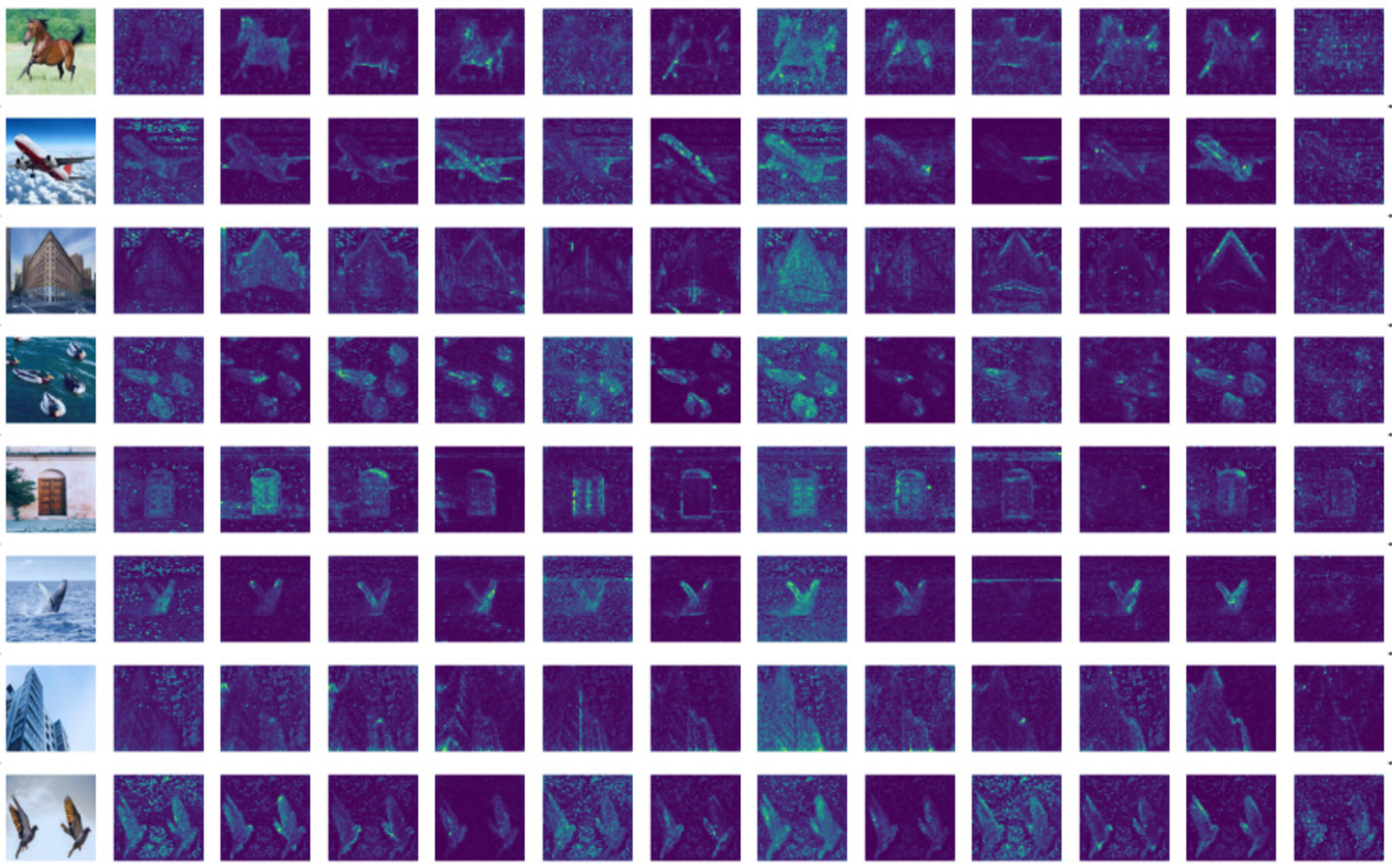
In particular, we examine what the attention maps for a given input reveal about the salient objects in the input image, i.e., which parts of the image provide the most globally-relevant information to the class token. One particular way to do this is to examine the component of the attention map where the class token is extracted as the query and removed from the value matrix, i.e., \(\vA _{2:, 1}^{k, L} \in \R ^{1 \times (n - 1)} = \R ^{1 \times N}\) or its transpose \(\va ^{k, L} = (\vA _{2:, 1}^{k, L})^{\top } \in \R ^{N}\). Notice that this vector \(\va ^{k, L}\), which we label as the “saliency vector at the \(k\)th attention head at layer \(L\),” has a value for every patch, \(1, \dots , N\), and we use this value to describe how relevant each patch is toward the global information. In particular for visualization’s sake we create a new image where each patch is replaced by its corresponding value in the saliency vector, showcasing the contribution of each patch; we call this image the “saliency map at the \(k\)th attention head at layer \(L\)”. To visualize the total relevance of each patch toward the global information across all heads, we can average the saliency vector, i.e., \(\tilde {\va }^{L} \doteq \frac {1}{K}\sum _{k = 1}^{K}\va ^{k, L}\) and expand into the average saliency map. The average saliency maps should highlight the relevant parts of the input image.

Object Detection and Segmentation. We can evaluate how the representations capture the fine-grained (i.e., smaller or more detailed) properties of the input by using them for semantic segmentation. Roughly, this means that we use the features to construct bounding boxes for all objects in the input. There are several ways to do this, and several ways to score the resulting bounding boxes compared to ground truth. Each combination of methods corresponds to a particular segmentation metric. We do not formally describe them here as they are not particularly insightful, but the DINO paper [CTM+21] and DINOv2 paper [ODM+23] contain references to all metrics that are used in practice.

8.2.6 Experimental Setup and Results

Since SimDINO is directly built upon DINO, we compare the optimal settings for DINO as given by their original paper [CTM+21] with the same settings applied to SimDINO [WZP+25] for a fair comparison.

Objective Function. We use \(10\) local views (i.e., \(M_{\loc } = 10\)) of resolution \(96 \times 96\) (i.e., \(S_{\loc } = 96\)) and \(2\) global views (i.e., \(M_{\glo } = 2\)) of resolution \(224 \times 224\) (i.e., \(S_{\glo } = 224\)) for all experiments. The corresponding portions of the original images cropped for local and global views are \(p_{\loc } \in [\frac {1}{20}, \frac {3}{10}]\) and \(p_{\glo } \in [\frac {3}{10}, 1]\) (chosen randomly per-view). The smaller edge size within the resized crops is \(S_{\rsz } = 256\), and the center crop (evaluation) view edge size is \(S_{\cc } = 224\). All of these settings apply to both DINO and SimDINO.

Model Architecture. For all inputs, we set the patch size to be \(16 \times 16\) (namely, \(P_{H} = P_{W} = 16\)). We use the small, base, and large models of the ViT [DBK+21] architecture as the embedding and backbone. The feature extractor is a three-layer MLP with a hidden size of \(2048\) and an output dimension of \(256\), followed by an \(\ell ^{2}\)-normalization, as specified in Section 8.2.3. For DINO architectures (i.e., not SimDINO architectures), the DINO head \(\vW \) is a matrix in \(\R ^{65536 \times 256}\), and the parameter \(\vmu \) is a vector in \(\R ^{65536}\).

Datasets and Optimization. For pre-training, both our DINO reproduction and SimDINO use the ImageNet-1K dataset across all methods. We use AdamW [LH17] as the optimizer, which is a very standard choice. We follow the following hyperparameter recommendations:

• The batch size is \(B = 1024\).
• The learning rate (for AdamW and the student model) has “base” value \(2 \times 10^{-3}\). In the first \(10\) epochs the learning rate linearly increases from \(0\) to the base value (i.e., at the \(i\)th epoch the learning rate is \((i/10) \cdot 2 \times 10^{-3}\), for \(1 \leq i \leq 10\)). Then over the next \(90\) epochs the learning rate decays via a so-called cosine schedule back down to \(0\). The definition of a cosine schedule is given in many places, including PyTorch documentation, and it is commonly used when training deep vision models.
• The weight decay (the W in AdamW) follows a cosine schedule from 0.04 to \(0.4\) over training.
• The EMA rate \(\nu \) follows a cosine schedule from \(0.996\) to \(1.0\) over training. Specifically for DINO, the centering EMA rate \(\rho \) is fixed at \(0.9\).
• Specifically for DINO, the teacher temperature \(\tau _{\teacher }\) is fixed at \(0.1\), while the student temperature \(\tau _{\student }\) linearly increases from \(0.04\) to \(0.07\) during the first \(30\) epochs and is fixed at \(0.07\) thereafter.

We use some (essentially information-preserving) data augmentations, such as flips, color jittering, Gaussian blur, and solarization, for each seen image during training, before taking the local and global views. The exact hyperparameters governing these are not listed here, but are referenced in the DINO paper [CTM+21].

For linear probing, the linear probe is usually trained using the AdamW optimizer with learning rate \(2 \times 10^{-4}\), weight decay \(0.01\), and batch size \(512\), but these are often modified on a case-by-case basis to minimize the loss.

Evaluation Results. In terms of downstream classification performance, we obtain the performance in Table 8.1. We observe that the performance of SimDINO is much higher than that of DINO under fair comparison. Also, it is much more stable: the prescribed settings of DINO cannot train a ViT-L(arge) model. On the other hand, Figure 8.10 shows visualizations of the average saliency maps in DINO and our simplified DINO, observing that the saliency maps look quite similar across models, indicating that the models learn features which are at least as good at capturing fine-grained details. The segmentation and object detection performances in Table 8.2 confirm this claim quantitatively, where SimDINO features show substantive improvement over those of DINO.

8.3 Weakly Supervised Image Representation via Text Binding

Another influential contrastive learning approach departs from purely visual comparisons and instead leverages the natural alignment between images and language. Rather than defining similarity solely through multiple views of the same image, this line of work exploits the fact that many images in the wild are accompanied by textual descriptions that provide weak semantic supervision. A prominent example of this paradigm is CLIP (Contrastive Language–Image Pretraining) [RKH+21a]. In CLIP, images and their corresponding captions are treated as positive pairs, while mismatched image–text pairs are treated as negatives. The learning objective encourages the representation of an image to be close to the representation of its associated caption, and far from captions of other images. By grounding visual representations in natural language, CLIP learns semantically rich features that capture high-level concepts beyond appearance alone.

8.3.1 Data

The data that we will use to explore the CLIP methodology are text-image pairs, rather than images alone. The original CLIP work constructed a large web-scale corpus of approximately 400 million text-image pairs collected from publicly available sources on the Internet. Each sample consists of an image and an associated natural-language string (e.g., a caption, title, or short description) that co-occurs with the image on the web, providing a weak and noisy form of supervision. To encourage broad coverage of visual concepts, the CLIP work describes building this dataset by searching for pairs whose text matches one of roughly 500,000 queries, and approximately balancing the results by including up to 20,000 pairs per query. This dataset is not publicly released, so most community replications and extensions of CLIP rely instead on open web-scale datasets of text-image pairs. The most common of which is the LAION [SBV+22] family: LAION-400M provides 400 million CLIP-filtered pairs, and LAION-5B scales this recipe to 5.85 billion pairs.

Because raw web-scraped pairs are often extremely noisy (e.g., images that do not match their associated text, boilerplate alt-text, spam, duplicates, or unsafe content), CLIP-style datasets are typically constructed with a post-processing pipeline that filters and cleans candidates before training. Typical methods include basic quality filters (e.g., dropping pairs with extremely short text or very small or corrupted images), language identification to retain captions in a target language, de-duplication, and the removal of potentially malicious content.

8.3.2 The CLIP Task and Objective

Our goal is to learn a good representation of the data. In the CLIP setting, however, the notion of “similarity” is not induced by two augmented views of the same image, but by the weak semantic supervision provided by natural-language descriptions. Concretely, we would like an image representation to be close to the representation of its associated caption, and far from captions of other images. Equivalently, if two images admit similar textual descriptions, their learned visual features should be similar, whereas images described by unrelated text should be separated in latent space.

We formalize the notion of “similarity” between representations using cosine similarity. Concretely, let \(f_{\theta }\) be an image encoder and \(g_{\plainphi }\) be a text encoder (whose architecture will be elaborated in the next section), both mapping into a common latent space \(\vZ \in \mathbb {R}^{d}\). Given an image \(\vX \in \cI \) and a text string \(\vT \in \cT \), we form normalized embeddings

Then the cosine similarity between embeddings is defined as:

Therefore, our objective is to maximize the cosine similarity between matched pairs and minimize it between mismatched pairs. To achieve that, we can use a simple symmetric cross-entropy loss as discussed in Section 7.4.2. Concretely, given a mini-batch of \(n\) text-image pairs \((\vX _i, \vT _i)_{i=1}^{n}\), we can define the loss as:

where \(\tau > 0\) is a temperature parameter that controls the sharpness of the softmax function.

8.3.3 Architecture: Vision Tower

The objective of CLIP is to learn both image and text representations in the same latent space. Accordingly, its architecture trains a vision encoder \(f_{\theta }: \cI \to \mathbb {R}^{d} \) and a text encoder \(g_{\plainphi }: \cT \to \mathbb {R}^{d} \) , also known as the “dual-tower architecture”.

In terms of architecture, most vision backbones can be used: for instance, convolutional networks such as ResNet [HZR+16a], as well as the Vision Transformer [DBK+21] (detailed in Section 8.2.3) are all valid choices for CLIP. In practice, the Vision Transformer is more commonly used due to better performance and versatility. Similarly to DINO, we take the class token feature \(\vz _{\cls }\) as the representation for each image: \(f_{\theta }(\vX ) = \vz _{\cls }\). This is because the class token is meant to aggregate global information about the entire image and is commonly used for downstream prediction tasks.

8.3.4 Architecture: Text Tower

The CLIP text tower \(g_{\plainphi }\) typically adopts a Transformer-based architecture similar to the Vision Transformer described earlier. The main difference lies in the embedding layer, which is used to convert the text sequence into a sequence of latent representations in the latent space \(\vZ \in \mathbb {R}^{d}\).

Embedding. Given a text sequence \(\vT \in \cT \) (e.g., a sentence or document), we embed it as a sequence of tokens in \(\R ^d\) using the map \(g_{\plainphi }^{\text {emb}}\), as follows.

1.

First, we tokenize \(\vT \) into a sequence of discrete symbols (subwords/characters) from a vocabulary \(\cV \) of size \(|\cV |\). Concretely, a tokenizer \(t^{\tok } : \cT \to \cV ^{N}\) produces a length-\(N\) token sequence⁵ \((\tau _{1},\dots ,\tau _{N})\), where \(\tau _i \in \cV \).

2.

We convert tokens to integer indices by a vocabulary map \(\cV \to \{1,\dots ,|\cV |\}\), yielding an index sequence \((s_{1},\dots ,s_{N})\). We place these indices into a matrix \(\vS \in \{0,1\}^{|\cV |\times N}\), where the \(i\)-th column is the one-hot vector \(\ve _{s_i}\).

3.

We then perform the following operation on \(\vS \) to project it to \(\R ^{d \times (N+1)}\):

\begin{equation} \vS \mapsto [\vz _{\cls }^{1}, \vW ^{\tok }\vS ] + \vE ^{\pos }. \tag{8.3.4} \end{equation}

This is the final output of \(g_{\plainphi }^{\text {emb}}\). Here we have three trainable parameters \(\vW ^{\tok }\), \(\vz _{\cls }^{1}\), and \(\vE ^{\pos }\) whose purpose is as follows:

• \(\vW ^{\tok } \in \R ^{d \times |\cV |}\) is a matrix whose \(j\)-th column is the learned embedding vector for the \(j\)-th vocabulary item. Thus \(\vW ^{\tok }\vS \in \R ^{d\times N}\) maps each discrete token to a continuous feature in \(\R ^{d}\).
• \(\vz _{\cls }^{1} \in \R ^{d}\) is a special classification (or summary) token. Heuristically, it is meant to aggregate global information about the entire sequence and is commonly used for downstream prediction tasks.
• \(\vE ^{\pos } \in \R ^{d \times n}\) is a positional encoding which distinguishes tokens at different positions. Since self-attention is permutation-equivariant in the token dimension, \(\vE ^{\pos }\) injects order information so that the overall map is not invariant to permutations of the tokens.

All parameters \(\vz _{\cls }^{1}, \vW ^{\tok }, \vE ^{\pos }\) are contained in the parameter set \(\theta \). The vocabulary \(\cV \) and tokenizer \(t^{\tok }\) are fixed.

Other components of the text tower, such as the backbone and the task-specific head, follow similar design choices as the image tower and are omitted for brevity. It is also worth noting that follow-up works have demonstrated substantial flexibility in the choice of CLIP’s text encoder: fixed text representations contained in large language models, and even simple bag-of-words features, can also be effective. We discuss these variants in Section 8.3.8.

8.3.5 Optimization Strategy

We train CLIP using a standard end-to-end stochastic optimization procedure (e.g. SGD with momentum, AdamW). Below we present a generic process.

At each timestep \(k\), we:

• Subsample paired data. Sample a minibatch of \(n\) paired examples

  \[ \{(\vX _i^{(k)}, \vT _i^{(k)})\}_{i=1}^{n} \subseteq \cX \times \cT , \]
  where \(\vX _i^{(k)}\) is an image and \(\vT _i^{(k)}\) is its associated text.

• Compute latent representations. For each pair \((\vX _i^{(k)}, \vT _i^{(k)})\), compute normalized embeddings using the vision and text encoders \(f_{\theta }\) and \(g_{\plainphi }\):

  \begin{equation} z_{\theta }^{I}(\vX _i^{(k)}) \doteq \frac {f_{\theta }(\vX _i^{(k)})}{\|f_{\theta }(\vX _i^{(k)})\|_2}, \qquad z_{\plainphi }^{T}(\vT _i^{(k)}) \doteq \frac {g_{\plainphi }(\vT _i^{(k)})}{\|g_{\plainphi }(\vT _i^{(k)})\|_2}. \tag{8.3.5} \end{equation}

• Compute CLIP loss. Compute the CLIP loss as defined in (8.3.3):

  \begin{equation} \displaystyle \hat {\cL }_{\text {CLIP}}^{(k)} \doteq -\frac {1}{n}\left ( \sum _{i=1}^{n} \frac {\exp (s(\vX _i^{(k)},\vT _i^{(k)})/\tau )}{\sum _{k=1}^{n}\exp (s(\vX _i^{(k)},\vT _k^{(k)})/\tau )} + \sum _{i=1}^{n} \frac {\exp (s(\vT _i^{(k)},\vX _i^{(k)})/\tau )}{\sum _{k=1}^{n}\exp (s(\vT _i^{(k)},\vX _k^{(k)})/\tau )} \right ). \tag{8.3.6} \end{equation}

• Compute gradients. Compute the gradients of the stochastic loss with respect to both parameter sets:

  \begin{equation} \nabla _{\theta }\hat {\cL }_{\text {CLIP}}^{(k)}(\theta ,\plainphi ), \qquad \nabla _{\plainphi }\hat {\cL }_{\text {CLIP}}^{(k)}(\theta ,\plainphi ). \tag{8.3.7} \end{equation}

• Update parameters. Apply one step of an optimization algorithm to \((\theta ,\plainphi )\), yielding the iteration

  \begin{equation} (\theta ^{(k+1)}, \plainphi ^{(k+1)}) \doteq \textsc {OptUpdate}^{(k)}\!\left ( (\theta ^{(k)}, \plainphi ^{(k)}); \nabla _{\theta }\hat {\cL }_{\text {CLIP}}^{(k)}, \nabla _{\plainphi }\hat {\cL }_{\text {CLIP}}^{(k)} \right ). \tag{8.3.8} \end{equation}

8.3.6 Evaluation Methodology

Since CLIP is architecture-agnostic, most standard evaluation protocols for vision and language encoders can be applied. For example, one can perform linear probing by training a lightweight classification head on top of the vision encoder to assess the quality of the learned representations in image classification tasks. Further, one can perform zero-shot classification without any additional training thanks to the dual-tower architecture of CLIP.

Recall that in a standard \(n\)-way image classification setup, we are given a dataset of images \(\{\vX _i\}_{i=1}^{N}\subseteq \cI \), each annotated with one of \(n\) class labels from the set \(\cL \doteq \{\ell _1,\ldots ,\ell _n\}\) (e.g., \(\ell _j \in \{\text {cat},\text {dog},\ldots \}\)). Our goal is to build a prediction pipeline \(P\), leveraging a pre-trained model, such that \(P:\cI \to \{1,\ldots ,n\}\) maps each image \(\vX _i\) to a predicted class index \(\hat {y}_i \doteq P(\vX _i)\). Writing the ground-truth class label as its index \(y_i \in \{1,\ldots ,n\}\), the (top-1) classification accuracy of \(P\) on this dataset is then computed as

In CLIP, we can use the text encoder \(g_{\plainphi }\) to build a text dictionary \(\vD \in \R ^{n\times d}\), whose \(j\)-th row is the normalized latent representation of the \(j\)-th class label. Concretely, for each class \(\ell _j \in \cL \), we construct a textual description (prompt) \(\vT _j\) (e.g., “a photo of a \(\ell _j\)”), and compute its normalized embedding \(\vz _j^T \doteq \frac {g_{\plainphi }(\vT _j)}{\|g_{\plainphi }(\vT _j)\|_2} \in \R ^{d}\). Stacking these row-wise yields

Given an image \(\vX _i \in \cI \), we compute its image representation via the vision encoder and normalize it as

We can then compute a similarity vector

whose \(j\)-th entry \(\vd _i[j]\) is the cosine similarity between the \(i\)-th image and the \(j\)-th class label in the shared latent space. By the CLIP training objective, images are encouraged to be more similar to their matching texts than to mismatched ones; hence a larger cosine similarity indicates closer alignment between \(\vX _i\) and class \(\ell _j\). Therefore, we predict the class index by

Finally, we can calculate the classification accuracy as mentioned above.

This zero-shot decision protocol is not limited to classification, but also applies naturally to retrieval tasks, where the goal is to return the most relevant items from a large database given a query (e.g., retrieve the most relevant images for a text query, or the most relevant texts for an image query). For instance, in text-to-image retrieval, instead of building a dictionary from class-name prompts, we build an image dictionary by encoding and normalizing all database images \(\{\vX _m\}_{m=1}^{M}\), stacking their embeddings into \(\vD \in \R ^{M\times d}\). Given a query text \(\vT \), we compute its normalized embedding \(\vz ^T \doteq g_{\plainphi }(\vT )/\|g_{\plainphi }(\vT )\|_2\), form similarity scores \(\vd \doteq \vD \vz ^T\in \R ^{M}\), and then rank images by these scores (equivalently, return the top-\(K\) indices).

8.3.7 Experimental Setup and Results

Next, we present results from the original CLIP paper comparing CLIP to a supervised ResNet baseline on several classic classification benchmarks. Across all benchmarks, CLIP is evaluated using the zero-shot classification protocol described in Section 8.3.6. Full details of the ResNet experimental setup are provided in [HZR+16a]; here, we briefly introduce the evaluation datasets and summarize CLIP’s training and evaluation settings relevant to these comparisons.

Evaluation Data.

• CIFAR-10 [KH+09]. CIFAR-10 is a widely used small-scale image classification benchmark consisting of 60,000 RGB images of size \(32\times 32\) across 10 classes (6,000 images per class). It is typically split into 50,000 training images and 10,000 test images.
• CIFAR-100 [KH+09]. CIFAR-100 has the same overall size and image resolution as CIFAR-10 (60,000 RGB \(32\times 32\) images with a 50,000/10,000 train/test split), but it is more challenging because it contains 100 fine-grained classes (600 images per class). The 100 classes are additionally grouped into 20 superclasses.
• PASCAL VOC 2007 (VOC2007) [EGW+10]. PASCAL VOC 2007 is a classic computer vision benchmark for object recognition, supporting tasks such as image classification, object detection, and segmentation. It focuses on 20 object categories (e.g., person, car, dog).
• ImageNet-1K [DDS+09a]. ImageNet-1K is a subset of ILSVRC 2012 containing 1,000 object classes. This subset includes 1,281,167 training images, 50,000 validation images, and 100,000 test images, and has played a central role in large-scale visual recognition and pretraining.

Model Setup. In the CLIP models demonstrated here, Vision Transformer is adopted as the vision encoder \(f_{\theta }\) and is instantiated as one of three ViT variants: ViT-B/32, ViT-B/16, or ViT-L/14. Here, \(\text {B}\) (“Base”) and \(\text {L}\) (“Large”) specify the transformer width/depth (e.g., ViT-B typically uses 12 transformer blocks with embedding dimension \(d=768\) and 12 attention heads, whereas ViT-L uses 24 blocks with \(d=1024\) and 16 heads), while the suffix \(/32\), \(/16\), and \(/14\) denotes the patch size in pixels used to patchify the input image . Smaller patch sizes (e.g., 16 or 14) yield more tokens per image at a fixed resolution, increasing compute but often improving accuracy due to finer spatial granularity.

Optimization Setup. All ViT-based CLIP models are trained for 32 epochs using the Adam optimizer with decoupled weight decay (i.e., AdamW-style regularization), where weight decay is applied to all parameters except gains and biases. The learning rate is decayed using a cosine schedule. The learnable temperature parameter \(\tau \) (used to scale the contrastive logits) is initialized to the equivalent of \(0.07\), and is clipped to prevent scaling the logits by more than 100, which is found necessary for training stability. Finally, training uses a very large mini-batch size of \(32{,}768\).

Results. Table 8.3 reports zero-shot top-1 accuracy of three CLIP ViT variants (B/32, B/16, L/14) and compares them to supervised ResNet-50 and ResNet-101 baselines. Across all four datasets, CLIP consistently outperforms the supervised ResNets. Scaling the CLIP backbone further yields additional gains, with ViT-L/14 reaching \(98.0\) on CIFAR-10, \(87.5\) on CIFAR-100, \(89.6\) on VOC2007, and \(83.9\) on ImageNet. Nevertheless, this table should be interpreted as a comparison between two systems rather than a controlled backbone ablation: CLIP benefits from large-scale image–text pretraining and is evaluated via zero-shot prompting, whereas the ResNet baselines rely on supervised pretraining and require labeled data to fit a probe on each benchmark. Thus, the consistent margins primarily demonstrate the strength of CLIP’s transferable representations under the zero-shot protocol, rather than establishing a purely architecture- or data-matched superiority of ViT over ResNet.

8.3.8 Simplified Extension: LIFT

While effective, CLIP exhibits several limitations. First, jointly training both a text encoder and an image encoder from scratch is computationally expensive, often requiring extremely large batches and massive datasets to reach strong alignment and downstream transfer. Second, models trained in this way can struggle with compositional understanding—capturing word order in text, spatial layout in images, and object–attribute or object–object relations—partly because retrieval-style contrastive supervision can reward shortcut solutions that downweight fine-grained compositional features. LIFT (Language–Image alignment with a Fixed Text encoder) [YWZ+25] revisits a core assumption underlying these pipelines: that optimal alignment demands joint end-to-end training of both encoders:

Instead, LIFT leverages the observation that modern large language models (LLMs) already produce highly informative text embeddings. Concretely, LIFT fixes a strong pretrained text encoder (e.g., one derived from or fine-tuned on an LLM), computes text embeddings offline, and trains only the image encoder to align to these fixed targets.

Architecture. LIFT retains the same dual-tower CLIP formulation in terms of a vision encoder and a text encoder that map into a shared latent space, but crucially differs in that the text tower is fixed and can be instantiated by any strong LLM-based text encoder \(g_{\plainphi }:\cT \to \R ^{d}\) to produce text embeddings, where \(\plainphi \) is not updated during training. In our implementation, we adopt the NV-Embed-V2 text encoder, for which the embedding dimension is \(d=4096\). Since the text tower \(g_{\plainphi }\) is fixed, we can pre-compute all text embeddings \(\{g_{\plainphi }(\vT )\}\) offline and, during training, only compute gradients and update the image encoder \(f_{\theta }\) online. The image tower \(f_{\theta }:\cI \to \R ^{d}\) follows the same structure as in Section 8.3.3, with the projection head output dimension set to \(d\) to match the dimension of the fixed text embedding space. Apart from fixing \(g_{\plainphi }\) and matching the projection dimension, the remaining components—including the contrastive loss and the optimization procedure—follow the same design principles as CLIP.

Evaluation Methodology. Compositional understanding is a known limitation of CLIP. We evaluate LIFT and CLIP on seven SugarCrepe [HZM+23] tasks, where each image \(\vX \) is paired with a positive (correct) caption \(\vT _{\text {pos}}\) and a negative caption \(\vT _{\text {neg}}\) constructed by adding, replacing, or swapping an object, attribute, or relation in \(\vT _{\text {pos}}\). See Figure 8.11 for some examples. Models are asked to identify the correct caption by comparing caption–image cosine similarities. Formally, for each sample \(i\in \{1,\dots ,N\}\), we compute the normalized embeddings

We then compute similarity scores via cosine similarities:

The model is considered correct on sample \(i\) if \(s_{i,\text {pos}} > s_{i,\text {neg}}\), and the overall compositional accuracy is

Experimental Results. As shown in Table 8.4, when trained on DataComp-1B, LIFT outperforms CLIP on all seven tasks with a 6.8% average accuracy gain. LIFT achieves significant gains on add attribute, replace attribute, and replace relation tasks. These improvements are strong evidence that LLM-based text encoders \(g_{\plainphi }\) capture more informative text representations that enable more accurate modeling of object–attribute associations and object–object relations. On the other hand, we can see LIFT shows relatively low accuracy on swap object and swap attribute compared to other SugarCrepe tasks. We attribute this limitation to the contrastive learning objective, which primarily focuses on aligning lower-order statistics. Addressing this challenge requires exploring more refined information-theoretic measures for language-image alignment, a key direction for future work.

8.4 Supervised Image Representation via Classification

In the previous sections, we have shown how to simplify some overly complex, often heuristically designed, learning objectives based on the principles of compression introduced in this book. However, objectives associated with some of the most popular learning tasks are already rather simple. In these cases, it is difficult to further simplify the objective. Thus, in this and future sections, we will focus on principled ways to modify the deep network architectures for a variety of tasks.

Let us first start with arguably the most classical task in machine learning: image classification, which is often used as a standard task to evaluate pattern recognition algorithms or deep network architectures. From our discussion of white-box architectures in Chapter 5, we only need a semantically meaningful task to learn good representations with white-box architectures. We will validate this idea in this section.

First, the dataset stays largely the same as Section 8.2.1. Both the training and test data consist of labeled images, i.e., image-label pairs \((\vX , \vy ) \in \R ^{C \times H \times W} \times \{0, 1\}^{N_{\cls }}\). We still apply various data augmentations (e.g., flips, Gaussian blurring, solarization, etc.) to each sample in each new batch.

8.4.1 Task and Objective

Unlike before, our task is not just to learn a good representation of the data, but also to simultaneously build a classifier. Formally, we have labeled data pairs \((\vX , \vy )\), where \(\vy \in \{0, 1\}^{N_{\cls }}\) is a one-hot vector denoting the class membership of \(\vX \). We consider a deterministic center crop view \(v_{\cc }\) of the input data \(\vX \) (cf Section 8.2.2). We want to jointly train a feature mapping \((f_{\theta }, f_{\theta }^{\ext })\) and a classification head \(h_{\theta }\), defined as follows:

where \((\vW ^{\head }, \vb ^{\head }) \in \R ^{N_{\cls } \times d} \times \R ^{N_{\cls }}\) are trainable parameters in the parameter set \(\theta \), such that the map \(\vX _{\cc } \mapsto \vp _{\theta }(\vX _{\cc }) \doteq h_{\theta }(\vz _{\theta }(\vX _{\cc }))\) predicts a smoothed label for the view \(\vX _{\cc } = v_{\cc }(\vX )\) of the input \(\vX \). The learning problem attempts to minimize the distance between \(\vp _{\theta }\) and \(\vy \) measured through cross-entropy:

8.4.2 The CRATE Architecture

The architecture that we use is the CRATE architecture, described in some detail in Chapter 5. The overall setup is similar to that of the regular transformer in Section 8.2.3, with a few changes. While the embedding step is the same as both DINO and SimDINO in Section 8.2.3, the feature extraction step is the same as SimDINO in Section 8.2.3 as it just extracts the feature corresponding to the class token, and the classification head is described in Section 8.4.1, the backbone architecture is different. Each layer takes the form

where the \(\MSSA _{\theta }^{\ell }\) and \(\ISTA _{\theta }^{\ell }\) blocks are as described in Chapter 5, namely:

• The \(\MSSA \) operator is multi-head-subspace-self-attention, defined as follows:

  \begin{equation} \MSSA _{\theta }^{\ell }(\vZ ) \doteq \vU _{\out }^{\ell }\mat {\SA ([\vU ^{1, \ell }]^{\top }\vZ , [\vU ^{1, \ell }]^{\top }\vZ , [\vU ^{1, \ell }]^{\top }\vZ )\\ \vdots \\ \SA ([\vU ^{K, \ell }]^{\top }\vZ , [\vU ^{K, \ell }]^{\top }\vZ , [\vU ^{1, \ell }]^{\top }\vZ )} + \vb _{\out }^{\ell }\vone _{n}^{\top } \tag{8.4.5} \end{equation}
  where \(\vU ^{k, \ell } \in \R ^{d \times p}\), \(\vU _{\out }^{\ell } \in \R ^{d \times Kp}\), and \(\vb _{\out }^{\ell } \in \R ^{d}\) are trainable parameters belonging to the parameter set \(\theta \), and (recall) the self-attention operator \(\SA \) is defined in (8.2.18).

• The \(\ISTA \) operator is the iterative-shrinkage-thresholding-algorithm operator, defined as follows:

  \begin{equation} \ISTA _{\theta }^{\ell }(\vZ ) \doteq \ReLU (\vZ - \beta (\vD ^{\ell })^{\top }(\vD ^{\ell }\vZ - \vZ ) + \beta \lambda \vone _{d}\vone _{n}^{\top }), \tag{8.4.6} \end{equation}
  so named because the map \(\vX \mapsto \ReLU (\vX - \beta \vD ^{\top }(\vD \vX - \vZ ) + \beta \lambda \vone _{d}\vone _{n}^{\top })\) is one step of the well-established ISTA algorithm to find an element-wise non-negative sparse representation for \(\vZ \) with respect to the complete dictionary \(\vD \) (cf Section 2.3).

We call this architecture CRATE, and a layer of the backbone is depicted in Figure 5.13. CRATE models, on top of being interpretable, are generally also highly performant and parameter-efficient.

8.4.3 Optimization

We train our classifier using a simple end-to-end stochastic optimization procedure, where we subsample data and views, compute the average loss and its gradient over these samples, and use an optimization algorithm to change the parameters. At each timestep \(k\), we:

• Subsample \(B\) different labeled samples \(\{(\vX _{b}^{(k)}, \vy _{b}^{(k)})\}_{b = 1}^{B} \subseteq \cI \times \{0, 1\}^{N_{\cls }}\).
• For each labeled sample \((\vX _{b}^{(k)}, \vy _{b}^{(k)})\), compute the central crop view \(v_{b, \cc }^{(k)}\) and apply it to \(\vX _{b}^{(k)}\) to get \(\vX _{b, \cc }^{(k)} \doteq v_{b, \cc }^{(k)}(\vX _{b}^{(k)})\).
• Compute the predictions \(\vp _{\theta }(\vX _{b, \cc }^{(k)}) \doteq (h_{\theta } \circ f_{\theta }^{\ext } \circ f_{\theta })(\vX _{b, \cc }^{(k)})\).

• Form the surrogate stochastic loss

  \begin{equation} \hat {\cL }_{\CE }^{(k)}(\theta ) \doteq \frac {1}{B}\sum _{b = 1}^{B}\CE (\vy _{b}^{(k)}, \vp _{\theta }(\vX _{b, \cc }^{(k)})). \tag{8.4.7} \end{equation}

• Compute one step of an optimization algorithm on \(\theta \), giving the following iteration:

  \begin{equation} \theta ^{(k + 1)} \doteq \textsc {OptUpdate}^{(k)}(\theta ^{(k)}; \nabla _{\theta }\hat {\cL }_{\CE }^{(k)}). \tag{8.4.8} \end{equation}

8.4.4 Evaluation Methodology

We use the same evaluation procedure as Section 8.2.5. To summarize, for all evaluations (as well as training) we use a center crop view \(v_{\cc }\) which reshapes the input image and takes a large central crop of size \((C, S_{\cc }, S_{\cc })\) where \(C\) is the number of channels in the input image. We can then do linear probing, attention map visualization, and detection/segmentation benchmarks, given the output of this view.

8.4.5 Experimental Setup and Results

Since CRATE is directly based on the transformer, we compare the optimal settings for ViT as given by [DBK+21; TCD+20] with the same settings applied to CRATE for a fair comparison.

Model Architecture. The center crop resizes the whole image so that the shorter edge is of size \(256\) (i.e., \(S_{\rsz } = 256\)) before taking a center crop of size \(224 \times 224\) (i.e., \(S_{\cc } = 224\)), both in evaluation and training. We take patch size \(16\) (i.e., \(P_{H} = P_{W} = 16\)). We use the tiny, small, base, and large models of the ViT [DBK+21] architecture as the embedding and backbone, swapping out the MHSA and MLP components for MSSA and ISTA, respectively, using the same number of heads and head dimension in the case of MSSA, and therefore reducing the number of training parameters drastically. For CRATE, we set \((\beta , \lambda ) = (1, 0.1)\).

Datasets and Optimization. For pre-training, we use the ImageNet-1K dataset. We use the LION optimizer [CLH+24] to pre-train both our ViT replication as well as CRATE. We set the base learning rate as \(2.4 \times 10^{-4}\), the weight decay as \(0.5\), and batch size as \(B = 2048\). Our learning rate schedule increases the learning rate linearly to the base learning rate over the first \(5\) epochs, and decreases to \(0\) using a cosine schedule over the next \(145\) epochs (training all models for \(150\) epochs each). For pre-training, we apply a usual regime of data augmentations (flips, Gaussian blurs, solarization, etc.) to the image data, and also add small noise to the labels (this is called label smoothing [MKH19]).

For linear probing, we use several evaluation datasets such as CIFAR10, Oxford-Flowers, and Oxford-IIT-Pets. We use the AdamW optimizer to train the linear probe, using learning rate \(5 \times 10^{-5}\), weight decay \(0.01\), and batch size \(B = 256\). We also apply the aforementioned data augmentations to the image data.

Experiment Results. Table 8.5 demonstrates that CRATE models achieve parity or improvement compared to the popular Vision Transformer (ViT) architecture at similar parameter counts, at least in terms of the linear separability of their features with respect to different classes. In terms of attention map fidelity, Figure 8.12 demonstrates a truly extraordinary result: without needing to train on any segmentation or object detection data, not only do the saliency maps effectively capture all relevant parts of the input image, the saliency maps self-organize to each correspond to a discrete set of concepts, even across samples and classes! This is the first system to do this, to the authors’ knowledge, and it can do this without using any extra data except for the image classification data. Table 8.6 confirms these qualitative insights quantitatively, showing significant improvement over ViTs trained in the same supervised classification setup.

8.5 Image Representation via Masked Autoencoding

In this section, we show how to apply the CRATE architecture to the image completion problem, also known as masked autoencoding (MAE), which can be viewed as a generalization of the low-rank matrix completion problem discussed in Chapter 2. Masked autoencoding, since its introduction in the deep learning context by [HCX+22], has been a staple and simple self-supervised representation learning method, which aims to endow each patch feature within \(\vZ _{\theta }\) with aggregate information as well as information about its neighbors, such that both the patch feature and aggregate features are rich sources of information for the whole sample.

The data we use for this task is the same as the image datasets discussed in Section 8.2.1. As usual, we still apply data augmentations to each sample in each new batch.

8.5.1 The MAE Task and Objective

As the name suggests, masked autoencoding involves a view \(v_{m}\) which, given an input, performs a random resized crop (cf Section 8.2.2) to turn the input image into a square image of size \((C, S_{\mask }, S_{\mask })\), then masks (i.e., sets to zero) a fixed percentage \(p_{\mask } \in [0, 1]\) of pixels in the input. For efficiency reasons⁶, the masking is done patch-wise, i.e., after embedding the whole image, \(p_{\mask }\) percentage of patches are set to zero. The goal of MAE is to train an encoder \(f_{\theta } \colon \cI \to (\R ^{d})^{*}\) and a decoder \(g_{\eta } \colon (\R ^{d})^{*} \to \cI \) that can reconstruct an input from its masking, i.e., writing \(\hat {\vX }_{\theta , \eta } \doteq g_{\eta } \circ f_{\theta }\), we have

Essentially this means that the features \(\vZ _{\theta }(\vX _{m})\) of the view \(\vX _{m} \doteq v_{m}(\vX )\) must contain information about the masked patches as well as the existing patches. From the perspective of the compression-based white-box models in Chapter 5, if a white-box autoencoder \((f_{\theta }, g_{\eta })\) succeeds at this task, it means that the learned subspaces and dictionaries perform a redundant encoding of the data such that it can reconstruct missing parts of the data from encoded other parts of the data. This means that information about each patch is stored in other patches. Therefore, each patch feature should contain both information about the patch and information about the statistics of the whole image. Thus, again, we expect that the representations should contain both local and global semantically relevant information, and therefore representations of different patches with similar local and global information should be related (i.e., on the same subspace or encoded together by a dictionary).

8.5.2 CRATE-Based MAE Architecture

We use a CRATE encoder and decoder, depicted in Figure 8.7, though of course it is possible to use a regular transformer encoder and decoder. Details follow.

The Encoder. The encoder is the same as the CRATE encoder in Section 8.4.2, with the caveat that there is no feature extractor \(f_{\theta }^{\ext }\). However, both the embedding \(f_{\theta }^{\emb }\) and the backbone \(f_{\theta }^{\backbone }\) are the same.

The Decoder Backbone. The decoder backbone is the CRATE decoder described in Chapter 6. For completeness, we describe it now. Given a feature sequence \(\vZ _{\theta }(\vX ) \doteq f_{\theta }(\vX ) \in (\R ^{d})^{*}\), we can process it using the decoder backbone \(g_{\eta }^{\backbone }\) as follows. The function \(g_{\eta }^{\backbone }\) is composed of \(L\) layers \(g_{\eta }^{\ell }\), i.e.,

The layer \(g_{\eta }^{\ell }\) has the following implementation. First, define \(\tilde {\vZ }_{\theta , \eta }^{1}(\vX ) \doteq \vZ _{\theta }(\vX )\). Then, we obtain

and \(g_{\eta }^{\ell }\) is defined such that \(g_{\eta }^{\ell }(\tilde {\vZ }_{\theta , \eta }^{\ell }) \doteq \tilde {\vZ }_{\theta , \eta }^{\ell + 1}(\vX )\). Here, the relevant concept is that \(g_{\eta }^{\ell }\) should learn an approximate inverse of \(f_{\theta }^{L + 1 - \ell }\), as discretizations of a forward- and reverse-time diffusion process, respectively. In particular, \(\tilde {\vD }^{\ell }\) should approximate \(\vD ^{L + 1 - \ell }\), and similarly, the \(\MSSA _{\eta }^{\ell }\) parameters should be similar to the parameters of \(\MSSA _{\theta }^{L + 1 - \ell }\). The output is \(\tilde {\vZ }_{\theta , \eta } \doteq \tilde {\vZ }_{\theta , \eta }^{L + 1}\).

The Un-embedding Module. To transform \(\tilde {\vZ }_{\theta , \eta }(\vX )\) back into an estimate for \(\vX \), we need to undo the effect of the embedding module \(f_{\theta }^{\emb }\) using the unembedding module \(g_{\eta }^{\unemb }\). As such, harkening back to the functional form of the embedding module in (8.2.13), i.e.,

it implies that our inverse operation \(g_{\eta }^{\unemb }\) looks like the following:

where \(g^{\unpatch }\) does the inverse operation of the unrolling and flattening operation that \(f^{\patch }\) does.⁷

This architecture is a white-box autoencoder \((f_{\theta }, g_{\eta })\) where (recall) \(f_{\theta } = f_{\theta }^{\backbone } \circ f_{\theta }^{\emb }\) and \(g_{\eta } = g_{\eta }^{\unemb } \circ g_{\eta }^{\backbone }\). In particular, we can use it to compute an estimate for a masked view \(\hat {\vX }_{\theta , \eta }(\vX _{m}) = (g_{\eta } \circ f_{\eta })(\vX _{m})\) which should approximately equal \(\vX \) itself.

8.5.3 Optimization

As in Section 8.4.3, we use a simple optimization setup: we sample images and masks, compute the loss on those samples and the gradients of this loss, and update the parameters using a generic optimization algorithm and the aforementioned gradients. For each timestep \(k\), we:

• Subsample \(B\) different samples \(\{\vX _{b}^{(k)}\}_{b = 1}^{B} \subseteq \cI \).
• For each sample \(\vX _{b}^{(k)}\), compute a different randomized resized crop and mask \(v_{b, m}^{(k)}\) and apply it to \(\vX _{b}^{(k)}\) to get \(\vX _{b, m}^{(k)} \doteq v_{b, m}^{t}(\X _{b}^{(k)})\).
• Compute the estimated autoencoding \(\hat {\vX }_{\theta , \eta }(\vX _{b, r}^{(k)}) \doteq (g_{\eta } \circ f_{\theta })(\vX _{b, r}^{(k)})\).

• Form the surrogate stochastic loss

  \begin{equation} \hat {\cL }_{\mathrm {MAE}}^{(k)}(\theta , \eta ) \doteq \frac {1}{B}\sum _{b = 1}^{B}\norm {\hat {\vX }_{\theta , \eta }(\vX _{b, r}^{(k)}) - \vX _{b}^{(k)}}_{F}^{2}. \tag{8.5.8} \end{equation}

• Compute one step of an optimization algorithm on \((\theta , \eta )\), giving the following iteration:

  \begin{equation} (\theta ^{(k + 1)}, \eta ^{(k + 1)}) \doteq \textsc {OptUpdate}^{(k)}(\theta ^{(k)}, \eta ^{(k)}; \nabla _{(\theta , \eta )}\hat {\cL }_{\mathrm {MAE}}^{(k)}). \tag{8.5.9} \end{equation}

8.5.4 Evaluation

This is the first autoencoder network we discuss in this chapter. We use the same center crop view \(v_{\cc }\) as in Sections 8.2.5 and 8.4.4, resizing the final image to a square with side length \(S_{\cc } = S_{\mask }\) pixels to match the shapes of the input images seen during training.

In addition to evaluating the masked autoencoding loss itself, it is also possible to evaluate the features \(\vZ _{\theta }(\vX _{\cc })\) of the view \(\vX _{\cc } \doteq v_{\cc }(\vX )\) of the data \(\vX \) directly. For attention map fidelity evaluation, obtaining \(\vZ _{\theta }(\vX _{\cc })\) is sufficient, but for linear probing we need to extract a summarized or aggregate feature from \(\vZ _{\theta }\). To do this, we can use a (parameter-free) feature extraction map that returns the feature corresponding to the class token, i.e.,

as in (for example) Sections 8.4.1 and 8.4.2. With this, we have a way to obtain aggregate features \(\vz _{\theta }(\vX _{\cc }) \doteq (f_{\theta }^{\ext } \circ f_{\theta })(\vX _{\cc })\), at which point we can perform linear probing, segmentation evaluations, and so on.

8.5.5 Experiments

Since CRATE-MAE is directly based on ViT-MAE, we compare the optimal settings for ViT-MAE as given by [HCX+22] with the same settings applied to CRATE-MAE for a fair comparison.

Model Architecture. During training, the masked crop \(v_{m}\) resizes the whole image so that the shorter edge is of size \(256\) (i.e., \(S_{\rsz } = 256\)) before taking a random crop of size \(224 \times 224\) (i.e., \(S_{\mathrm {mask}} = 224\)), and masking \(p_{\mathrm {mask}} = \frac {3}{4}\) of the patches. We take patch size \(16\) (i.e., \(P_{H} = P_{W} = 16\)). We use the small and base variants of the ViT-MAE architecture as the embedding and backbone for both the encoder and decoder, swapping out the MHSA and MLP components for MSSA, ISTA, and linear layers, respectively. We use the same number of heads and head dimension in the case of MSSA. However, the original ViT-MAE uses an encoder which uses nearly all the total layers and a decoder which only uses a few layers; we allocate half the total number of layers (which stays the same from ViT-MAE to CRATE-MAE) to our encoder and decoder, as suggested by the conceptual and theoretical framework in Chapter 6. For CRATE-MAE we set \((\beta , \lambda ) = (1, 0.1)\).

Datasets and Optimization. For pre-training, we use the ImageNet-1K dataset. We use the AdamW optimizer to pre-train both our ViT-MAE replication as well as CRATE-MAE. We set the base learning rate as \(3 \times 10^{-5}\), the weight decay as \(0.1\), and batch size as \(B = 4096\). Our learning rate schedule increases the learning rate linearly to the base learning rate over the first \(40\) epochs, and decreases to \(0\) using a cosine schedule over the next \(760\) epochs (training all models for \(800\) epochs each). For pre-training, we apply the usual regime of data augmentations (flips, Gaussian blurs, solarization, etc) to the image data.

For linear probing, we use several evaluation datasets such as CIFAR10, CIFAR100, Oxford-Flowers, and Oxford-IIT-Pets. For linear probing, we precompute the features of all samples in the target dataset and apply a fast linear regression solver, e.g., from a standard package such as Scikit-Learn.

Experiment Results. Table 8.7 demonstrates that CRATE-MAE models achieve, roughly speaking, parity with the popular ViT-MAE architecture at similar parameter counts, and also that the feature learning performance (as measured by performance on downstream classification tasks) increases with scale. Meanwhile, Figure 8.14 demonstrates that the encoder saliency maps (and therefore the fine-grained features learned by the encoder) indeed isolate and highlight the key parts of the input image.

8.6 Image Generation via Auto-Encoding and Sampling

In the previous section, we have introduced masked autoencoding (MAE) as one approach to learn an autoencoding of natural images \(\x \sim p(\x )\):

where \(\z = f(\x )\) is certain feature space. Such an autoencoding is designed to learn correlation, or co-occurrence, among patches of a natural image.

However, MAE does not enforce the (distribution of) learned features \(\z \) to have any explicit structures or properties, which can be very important if we want to use the so-learned features for certain subsequent tasks such as recognition or controlled generation. In addition, the simple MMSE loss used for image completion does not necessarily respect the possible nonlinear structures in the image manifold and typically generate an expected value, hence usually blurred version, for the missing image patches, as we have shown in Figure 7.8 in the previous Chapter 7.

Hence, in this section, we will introduce some other methods to learn representations for (the distribution of) natural images via auto-encoding that aim, to large extent, to remedy the above two issues. More precisely, we want the distribution of the encoded features to have certain desired structures and images decoded from such features are much more faithful to the distribution of natural images – that is, of much better visual quality.

8.6.1 Variational Auto-Encoding of Imagery Data

As we have introduced in Section 6.1.4 of Chapter 6, variational auto-encoding is a method that aims to promote the distribution of learned features \(\z \) and the conditional distributions between \(\x \) and \(\z \) to be more Gaussian like.⁸

Here we introduce a popular implementation of a VAE for imagery data, following the perceptual compression model leveraged in Stable Diffusion [RBL+22]. The key idea is to train an autoencoder that maps high-resolution images into a low-dimensional latent space, while imposing a KL-regularization on the latent distribution to encourage it to be close to a standard Gaussian \(\mathcal {N}(\boldsymbol {0}, \boldsymbol {I})\). This latent space can subsequently serve as an efficient arena for downstream generative models such as latent diffusion. Both the encoder and decoder are jointly trained end-to-end. We outline the details as follows.

The Encoder (\(\mathcal {E}\)). The encoder \(\mathcal {E}\) maps an input RGB image \(\x \in \mathbb {R}^{H \times W \times 3}\) into a low-dimensional latent space. Its architecture, adopted from [ERO21], is a fully convolutional network. It begins with an input convolution that projects the 3-channel RGB input into a feature map with a base channel count of \(128\). This is followed by four stages, each consisting of two ResNet blocks [HZR+16b]. The channel dimension is scaled by multipliers \((1, 2, 4, 4)\) across stages, yielding feature maps with \(128, 256, 512, 512\) channels, respectively. Spatial downsampling by a factor of \(2\times \) is performed between consecutive stages via strided convolutions, resulting in three downsamplings and an overall downsampling factor of \(f = 2^3 = 8\). After the four stages, a middle block consisting of two additional ResNet blocks further refines the features. Finally, an output convolution projects the features to \(2c\) channels, which are split into the two quantities that parameterize the latent distribution (described below).

Crucially, unlike a standard autoencoder, the encoder does not output a single deterministic latent vector. Instead, it parameterizes a diagonal Gaussian posterior \(q(\z | \x ) = \mathcal {N}(\boldsymbol {\mu }, \boldsymbol {\sigma }^2 \boldsymbol {I})\) by outputting two quantities:

• A mean \(\boldsymbol {\mu } = \mathcal {E}_\mu (\x ) \in \mathbb {R}^{h \times w \times c}\), and
• A log-variance \(\log \boldsymbol {\sigma }^2 = \mathcal {E}_\sigma (\x ) \in \mathbb {R}^{h \times w \times c}\).

The latent representation is then obtained via a so called reparameterization trick [KW13b]:

where \(\hada \) denotes element-wise multiplication. This formulation enables gradient-based optimization through the stochastic sampling step.

The Decoder (\(\mathcal {D}\)). The decoder \(\mathcal {D}\) learns the reverse mapping from the latent space back to the pixel space, producing the reconstructed image \(\tilde {\x } = \mathcal {D}(\z ) \in \mathbb {R}^{H \times W \times 3}\). Its architecture is approximately symmetric to the encoder: an input convolution first projects the \(c\)-channel latent into the feature space, followed by a middle block of two ResNet blocks. Then, four stages—each with two ResNet blocks—progressively upsample the spatial resolution, with the channel dimensions mirroring those of the encoder in reverse order (\(512, 512, 256, 128\)). A final output convolution maps the features back to 3 RGB channels. Both the encoder and decoder architectures follow the convolutional design introduced in [ERO21].

Data

We assume access to a dataset \(\mathcal {D} = \{\x _i\}_{i=1}^N\) of samples from the original data distribution. Each sample is an image of the form \(\x \in \mathbb {R}^{H \times W \times 3}\), where \(H\) and \(W\) are the height and width, respectively. In [RBL+22], the autoencoder is trained on the OpenImages dataset with images cropped to \(256 \times 256\) resolution.

Given the downsampling factor \(f = 8\) and latent channel count \(c = 4\), the encoder maps each input image to a latent tensor \(\z \in \mathbb {R}^{H/f \times W/f \times c}\). For the default training resolution, this yields a latent of size \(32 \times 32 \times 4\). At inference time, the autoencoder generalizes to other resolutions; for example, a \(512 \times 512 \times 3\) input is encoded into a \(64 \times 64 \times 4\) latent.

Objective and Evaluation Metrics

To train the VAE, our goal is to jointly optimize the encoder \(\mathcal {E}\) and decoder \(\mathcal {D}\) such that the reconstructed data \(\tilde {\x } = \mathcal {D}(\mathcal {E}(\x ))\) is as close as possible to the original data \(\x \), while regularizing the latent distribution to be close to a standard Gaussian prior. An empirically effective choice of the reconstruction loss is a weighted combination of L1, LPIPS [ZIE+18], and adversarial losses as in GAN [GPM+14b]. Additionally, a KL divergence term is included to regularize the latent space. Formally, the training objective can be expressed as:

where \(\theta _{\mathcal {E}}\) and \(\theta _{\mathcal {D}}\) are the parameters of the encoder and decoder, respectively, and \(\lambda _1, \lambda _2, \lambda _3\) are hyperparameters that balance the contributions of each loss term. The first three terms enforce sample-wise consistency in the same manner as the reconstruction objectives in Section 8.6.2. The fourth term—the KL divergence between the encoder posterior \(q(\z | \x ) = \mathcal {N}(\boldsymbol {\mu }, \boldsymbol {\sigma }^2 \boldsymbol {I})\) and the standard Gaussian prior \(p(\z ) = \mathcal {N}(\boldsymbol {0}, \boldsymbol {I})\)—regularizes the latent space. For a diagonal Gaussian posterior, this admits a closed-form expression:

where \(d = h \times w \times c\) is the total dimensionality of the latent space.

The implementation detail from [RBL+22] is that the KL weight \(\lambda _3\) is set to a very small value (\(\approx 10^{-6}\)). This is because the primary purpose of the KL term here is not to enable unconditional sampling from the latent space (as in a traditional VAE), but rather to prevent the latent space from developing arbitrarily high variance, which would degrade the signal-to-noise ratio for downstream models operating in this space.

For evaluation, we measure the reconstruction quality by computing the FID score [HRU+17b] on the reconstructed images from the ImageNet-1k validation set, denoted as rFID. A lower rFID indicates better reconstruction quality.

8.6.2 Representation Auto-Encoding of Imagery Data

As discussed in Chapter 4, learning structured representations of the data is crucial for many downstream tasks. In visual representation learning, this is often achieved by self-supervised learning methods such as DINO [CTM+21] and SimDINO (studied in Section 8.2). In Chapter 6, we posit that a good representation of data should be effectively decoded back into the original data space. This requires a consistent auto-encoding framework that can accurately reconstruct the original data from its learned representation. It is then natural to ask: is the representation learned by methods like DINO consistent and can it be effectively decoded in an auto-encoding framework?

To find out, we can train a representation auto-encoder (RAE) that consists of an pretrained representation encoder (e.g. DINO) and a trainable decoder, following the work:

The encoder \(f\) maps an input sample \(\x \) to its learned representation \(\z = f(\x )\), while the decoder \(g\) maps the representation back to the original data space \(\x '=g(\z )\). As detailed in Chapter 6, one simple objective is to impose sample-wise consistency by training the decoder to minimize the reconstruction loss between the original data \(\x \) and the reconstructed data \(\x '\). We outline the details as follows.

The Encoder. We use a pretrained representation encoder \(f \colon \cX \to \cZ \) that maps an input data sample \(\x \in \cX \) to its learned representation \(\z = f(\x ) \in \cZ \). The encoder is kept frozen during training. Here, we assume a ViT-based encoder, as introduced in Section 8.2.3.

The Decoder. For architectural simplicity, we use a trainable ViT-based decoder \(g \colon \cZ \to \cX \) that maps the learned representation \(\z \) back to the original data space, producing the reconstructed data \(\x ' = g(\z )\).

Data

We assume access to a dataset \(\cD = \{\x _i\}_{i=1}^N\) of samples from the original data distribution \(\cX \). Each sample is an image of the form \(\x \in \R ^{3 \times H \times W}\), where \(H\) and \(W\) are the height and width, respectively. The encoder \(f\) is set to a patch size of \(p_e\) and feature dimension of \(d\). Consequently, for each input image \(\x \), we would obtain \(N = HW/p_e^2\) tokens of dimension \(d\). The decoder \(g\) with patch size \(p_d\) then maps these visual tokens back to reconstruct \(\x ' \in \R ^{3 \times H\frac {p_d}{p_e} \times W\frac {p_d}{p_e}}\) in the original pixel space. By default, we set \(p_d = p_e\) to ensure that the reconstructed image has the same resolution as the original image.

Objective and Evaluation Metrics

To train RAE, our goal is to train a decoder \(g\) such that the reconstructed data \(\x ' = g(f(\x ))\) is as close as possible to the original data \(\x \). This can be achieved by minimizing a sample-wise consistency loss over the dataset \(\cD \). An empirically effective choice of the loss function is a weighted combination of L1, LPIPS [ZIE+18] ⁹, and adversarial losses as in GAN [GPM+14b]. Formally, the training objective can be expressed as:

where \(\theta \) are the parameters of the decoder \(g\), and \(\lambda _1, \lambda _2\) are hyperparameters that balance the contributions of each loss term.

For evaluation, we measure the reconstruction quality by computing the FID score [HRU+17b] on the reconstructed images from the ImageNet-1k validation set, denoted as rFID. A lower rFID indicates better reconstruction quality.

Experimental Results

We can compare RAEs trained on different pretrained encoders, including DINOv2, MAE, and SigLIP2. As a baseline, we also consider a vanilla variational autoencoder (VAE) trained directly on the image pixels without any pretrained encoder. One popular choice is SD-VAE. RAE decoders are trained on the ImageNet-1K training set and evaluated on the ImageNet-1K validation set. The results are summarized in Table 8.8d. From Table 8.8b, we can see that RAEs with pretrained encoders outperform SD-VAE in reconstruction quality. Furthermore, larger decoder sizes lead to improved reconstruction quality, as shown in Table 8.8b, while remaining more efficient than VAEs. Table 8.8c shows that the reconstruction quality is stable across different sizes of the DINO encoders. Finally, Table 8.8d demonstrates that RAEs also retain high-quality representations, achieving much higher linear probing accuracy compared to VAEs.

To complement the quantitative metrics in Table 8.8d, Figure 8.15 provides a visual comparison of reconstructions. RAE reconstructions preserve fine-grained textures, object boundaries, and semantic details as faithfully as the SD-VAE baseline, consistent with its better rFID scores.

8.6.3 Sampling from Learned Representations via Denoising

Once we have learned a consistent and structured representation of the distribution of natural images, say via VAE or RAE, we typically like to efficiently generate samples \(\z \in \cZ \) from the learned representation distribution so that we can regenerate the natural images associated with these samples via the learned decoder \(\hat {\x } = g(\z ) \in \cX \). This auto-encoding process is illustrated by the top half of Figure 1.27 in Chapter 1.

To learn hence sample the distribution of the features \(\z \) in the latent space \(\cZ \), we can leverage the denoising and diffusion method introduced in Chapter 3. Concretely, suppose \(p(\z )\) is the distribution of the learned features \(\z \) in the feature space. We may learn a denosing process that, starting from an initial standard Gaussian distribution \(\vg \sim \cN (0, \vI )\), converges to this distribution \(p(\z )\). Following the method introduced in Chapter 3, we want to learn a denoiser \(\bar {\z }\) such that it iteratively denoises a sample from the initial distribution \(\cN (0, \vI )\) to the target distribution of the learned representations \(p(\z )\). This process is illustrated by the bottom half of Figure 1.27 in Chapter 1.

Here to learn the denoising, let us take the simple case of flow matching introduced in Chapter 3. We can define the denoiser as a time-dependent vector field \(\bar {\z }_{\theta }(t, \z _t)\) parameterized by \(\theta \) that transforms a sample from the initial distribution to the target distribution over time \(t \in [0, 1]\). Here, \(\z _t\) is an interpolation between \(\z _0\) and \(\z _1\) at time \(t\):

where \(\z _0 \sim p(\z )\) is a sample from the learned representation distribution and \(\z _1 \sim \cN (0, \vI )\). The training objective for the denoiser can then be expressed as:

Typically, the denoising vector field \(\bar {\z }_{\theta }(t, \z _t)\) are modeled by a deep network. Popular choices of the deep network can be either a U-Net or a diffusion image transformer (DiT). Below we provide more details about how they can be implemented in practice.

8.6.4 Realizing Denoising with a U-Net

The dominant architecture for implementing the denoising network \(\boldsymbol {\epsilon }_\theta \) in diffusion models has been the U-Net [RFB15a], an encoder-decoder convolutional network with skip connections originally developed for biomedical image segmentation. Ho et al. [HJA20] first adopted the U-Net as the backbone for Denoising Diffusion Probabilistic Models (DDPM), establishing it as the default architecture for the field. Subsequently, Dhariwal and Nichol [DN21a] conducted a systematic series of architectural ablations that substantially improved the U-Net design, producing what they call the Ablated Diffusion Model (ADM). Their improved model was the first diffusion model to surpass GANs in sample quality on ImageNet. Building on these foundations, Rombach et al. [RBL+22] moved the U-Net from pixel space into the latent space of a pretrained VAE (Section 8.6.1) and introduced cross-attention layers for flexible multi-modal conditioning, giving rise to the Latent Diffusion Model (LDM) that underpins Stable Diffusion. In this section, we trace the evolution of the U-Net backbone through these three stages, before discussing the architectural limitations that have motivated the recent transition to transformer-based alternatives (Section 8.6.5).

Encoder-Decoder Structure with Skip Connections. The U-Net follows an encoder-decoder structure. The encoder progressively downsamples the input through a series of resolution stages, extracting features at multiple spatial scales; the decoder then upsamples these features back to the original resolution to produce the output prediction. The distinguishing feature of the U-Net is its skip connections: at each resolution level, the encoder feature map is concatenated channel-wise to the corresponding decoder feature map. This allows the decoder to combine coarse, semantically rich features from the bottleneck with fine-grained spatial details from earlier encoder layers, which is essential for producing spatially precise predictions.

In the DDPM U-Net [HJA20], the architecture begins with an input convolution that projects the noised input into a feature space with a base channel count (e.g., 128). The encoder then proceeds through multiple resolution stages—four for \(32 \times 32\) inputs, or six for \(256 \times 256\) inputs—where each stage consists of two convolutional residual blocks. Spatial downsampling by a factor of \(2\times \) is performed between consecutive stages via strided convolutions. Self-attention layers are inserted at the \(16 \times 16\) resolution level between the convolutional blocks, providing limited long-range modeling at low resolution. At the bottleneck (the lowest resolution), a middle block with additional residual blocks and self-attention further refines the features. The decoder mirrors the encoder: residual blocks at each resolution level followed by upsampling via transposed convolutions, with skip connections concatenating the corresponding encoder activations. The architecture uses group normalization [WH20] throughout, replacing the weight normalization from which the design originates.

When the U-Net operates in pixel space, its input and output are the noised image \(\x _t \in \mathbb {R}^{H \times W \times 3}\) and the predicted noise \(\hat {\boldsymbol {\epsilon }} \in \mathbb {R}^{H \times W \times 3}\), respectively. When operating in the latent space of a pretrained VAE (as in LDM), the input becomes \(\z _t \in \mathbb {R}^{h \times w \times c}\) and the output is \(\hat {\boldsymbol {\epsilon }} \in \mathbb {R}^{h \times w \times c}\), with \(h = H/f\), \(w = W/f\) as defined in Section 8.6.1.

Timestep Conditioning via Adaptive Group Normalization. The denoising network must be conditioned on the diffusion timestep \(t\) so that it can adapt its behavior across different noise levels. Following the positional encoding scheme from the Transformer [VSP+17b], the timestep \(t\) is first mapped to a sinusoidal frequency embedding:

where \(d_e\) is the embedding dimension and \(i\) indexes its entries. This embedding is then passed through a small MLP (typically two linear layers with a nonlinearity) to produce a timestep vector \(\boldsymbol {e}_t \in \mathbb {R}^{d_e}\).

Rather than simply concatenating \(\boldsymbol {e}_t\) to the input, the U-Net injects the timestep information into every residual block via Adaptive Group Normalization (AdaGN) [DN21a]. After the first convolution within each residual block, a group normalization operation is applied, followed by an affine modulation whose scale and shift parameters are regressed from the timestep embedding:

where \(\boldsymbol {h}\) denotes the intermediate feature map, \([\boldsymbol {y}_s, \boldsymbol {y}_b] = \mathrm {Linear}(\boldsymbol {e}_t)\) are the scale and shift vectors obtained from a linear projection of the timestep embedding, and \(\hada \) denotes element-wise multiplication. This mechanism is analogous to adaptive instance normalization [DSK17] and FiLM conditioning [PSV+18], and allows each layer to modulate its activations based on the current noise level. Ablation experiments in [DN21a] show that removing AdaGN degrades FID by over 2 points, confirming its importance.

For class-conditional generation, a class embedding \(\mathrm {Embed}(c)\) (a learned lookup table) is simply added to the timestep embedding before injection, so that \(\boldsymbol {e}_t\) is replaced by \(\boldsymbol {e}_t + \mathrm {Embed}(c)\) in Eq. (8.6.10). This mechanism is lightweight but limited to categorical labels; richer conditioning modalities such as text require the cross-attention mechanism introduced in Section 8.6.4.0.

Architecture Improvements: From DDPM to ADM

Dhariwal and Nichol [DN21a] conducted a systematic ablation study to identify which architectural modifications most improve sample quality. Starting from the baseline DDPM U-Net [HJA20], they explored the following changes on ImageNet \(128 \times 128\): (a) expanding self-attention from the \(16 \times 16\) resolution to three resolutions (\(32 \times 32\), \(16 \times 16\), \(8 \times 8\)); (b) increasing the number of attention heads, using 64 channels per head to better match the Transformer convention; (c) adopting the BigGAN [BDS19] residual block for both upsampling and downsampling, which improves gradient flow; and (d) including the AdaGN conditioning layer (described above) in every residual block by default. All of these changes improve FID, and their effects compound positively. The resulting model, which they name ADM, serves as the new default U-Net design for subsequent work.

In addition to architectural improvements, Dhariwal and Nichol introduced classifier guidance as a mechanism for trading off sample diversity against fidelity. A classifier \(p_\phi (c|\z _t, t)\) is trained on noisy images, and its gradients are used to steer the sampling trajectory toward high-probability regions of the desired class:

where \(s > 1\) is a guidance scale that sharpens the effective class distribution. With this technique, ADM achieved a state-of-the-art FID of 4.59 on class-conditional ImageNet \(256 \times 256\), surpassing the long-standing GAN benchmark of BigGAN-deep (FID 6.95) for the first time. The guided model (ADM-G) further improved FID to 3.94 when combined with an upsampling stack (ADM-U).

The main drawback of classifier guidance is that it requires training a separate classifier on noisy images. This limitation was subsequently addressed by classifier-free guidance [HS22b], which avoids the external classifier entirely by jointly learning conditional and unconditional denoising within a single model—a technique we describe in detail in Section 8.6.5.

The U-Net in Latent Diffusion (Stable Diffusion)

While ADM operates directly in pixel space, Rombach et al. [RBL+22] observed that much of the computational burden is spent modeling perceptually irrelevant high-frequency details. Their key idea is to separate perceptual compression from generative modeling: a pretrained autoencoder (Section 8.6.1) first compresses the image into a low-dimensional latent space, and the diffusion model then operates entirely within this latent space. For a \(256 \times 256\) image with downsampling factor \(f = 8\), the U-Net processes a \(32 \times 32 \times 4\) latent tensor rather than a \(256 \times 256 \times 3\) pixel tensor—a reduction of roughly \(48\times \) in spatial elements. This yields a speedup of at least \(2.7\times \) in both training and sampling throughput while improving FID.

Beyond computational savings, the latent diffusion framework introduces a general-purpose cross-attention conditioning mechanism that enables the U-Net to condition on arbitrary modalities such as text prompts, semantic maps, or bounding boxes. In brief, a domain-specific encoder \(\tau _\theta \) maps the conditioning input \(\boldsymbol {y}\) into an intermediate representation \(\tau _\theta (\boldsymbol {y}) \in \mathbb {R}^{M \times d_\tau }\), which is then injected into the U-Net at multiple resolution levels via cross-attention layers: the image features serve as queries while the conditioning embeddings serve as keys and values, allowing each spatial location to attend to relevant parts of the conditioning signal. We defer the full mathematical description of this cross-attention mechanism and the conditional training objective to Section 8.7.2.

In Stable Diffusion [RBL+22], the text encoder \(\tau _\theta \) is instantiated as the pretrained CLIP ViT-L/14 model [RKH+21b], which maps text prompts to a sequence of token embeddings. The U-Net itself retains the ADM improvements—BigGAN residual blocks, attention at three resolution levels, AdaGN for timestep injection—and additionally interleaves cross-attention layers at these same resolution levels for text conditioning. The full model contains approximately 860M parameters in the U-Net and 123M in the text encoder.

Limitations of the U-Net Architecture

Despite its success, the U-Net has several limitations that have motivated alternative backbones. First, scaling a U-Net is cumbersome: its encoder-decoder structure involves many coupled design choices (channel multipliers, attention placement, up/downsampling block types), and it is unclear how to allocate additional compute optimally. In contrast, the plain Transformer scales along two simple axes, depth and width, and exhibits well-characterized scaling laws based on empirical studies [KMH+20]. Second, the U-Net’s convolutional layers encode a strong spatial inductive bias (locality, translation equivariance) that helps in low-data regimes but limits long-range modeling on large datasets. Self-attention partially addresses this, yet in standard U-Net designs it is applied only at low-resolution stages due to its quadratic cost, leaving high-resolution features entirely local. Third, the U-Net is a image-specific architecture that does not readily generalize so well to other modalities. The Transformer, having proven effective across language, vision, audio, and multimodal settings [VSP+17b], offers a unified backbone that can leverage cross-domain scaling insights.

These considerations motivated the Diffusion Transformer (DiT) [PX23], which replaces the U-Net entirely with a plain Transformer operating on latent patches. As we describe in Section 8.6.5, DiT matches and surpasses the best U-Net-based models while exhibiting cleaner scaling behavior (Gflops–FID correlation of \(-0.93\)) and a simpler architecture.

8.6.5 Realizing Denoising with a Diffusion Transformer

An alternative to the U-Net for implementing the denoising network \(\boldsymbol {\epsilon }_\theta \) is the Diffusion Transformer (DiT) [PX23], which replaces convolutions entirely with transformer blocks. The key insight is that the U-Net’s spatial inductive bias is not crucial to the performance of diffusion models: a standard transformer operating on sequences of latent patches can match and surpass the U-Net while inheriting the favorable scaling properties of the transformer architecture class [VSP+17b]. Unlike the U-Net, the DiT has no explicit spatial inductive bias—all spatial structure is learned from data. This generality enables the same architecture to handle images, video, and other modalities with minimal modification.

DiT operates within the latent space of a pretrained VAE (Section 8.6.1), making the complete image generation pipeline a hybrid architecture: a convolutional VAE for perceptual compression and a transformer-based DDPM for generative modeling. Following the Vision Transformer (ViT) [DBK+21], the input latent is divided into patches and linearly embedded as a token sequence. We describe the architecture in detail below.

Patchify and Positional Encoding. The input to DiT is a noised latent \(\z _t \in \mathbb {R}^{h \times w \times c}\), where \(h = H/f\) and \(w = W/f\) are the spatial dimensions of the latent space defined by the VAE encoder (e.g., \(32 \times 32 \times 4\) for \(256 \times 256\) images with \(f = 8\), \(c = 4\)). The first layer, called patchify, partitions \(\z _t\) into a grid of non-overlapping patches of size \(p \times p\) and linearly embeds each patch into a \(d\)-dimensional token representation. This produces a sequence of

tokens in \(\mathbb {R}^d\). Standard sinusoidal positional embeddings (the sine-cosine variant from ViT) are added to each token to encode spatial position. The patch size \(p\) is a key design parameter: halving \(p\) quadruples \(T\) and thus at least quadruples the total Gflops of the transformer, while leaving the parameter count essentially unchanged. In [PX23], the design space includes \(p \in \{2, 4, 8\}\); the finest setting \(p = 2\) yields the best generation quality.

DiT Block with adaLN-Zero. After patchification, the token sequence is processed by a stack of \(N\) transformer blocks. Each block follows the standard transformer structure [VSP+17b]: layer normalization, multi-head self-attention (MHSA), a second layer normalization, and a pointwise feedforward network (MLP with GELU activations).

The central design question is how to inject the conditioning information—the diffusion timestep \(t\) and the class label \(c\)—into each block. Peebles and Xie [PX23] compare four strategies: (1) in-context conditioning, which appends \(t\) and \(c\) as extra tokens in the input sequence; (2) cross-attention, which introduces an additional multi-head cross-attention layer that attends to the conditioning embeddings; (3) adaptive layer normalization (adaLN), which regresses the scale and shift parameters of each layer normalization from the conditioning signal; and (4) adaLN-Zero, which extends adaLN with an additional gating mechanism initialized to zero. Among these, adaLN-Zero achieves the lowest FID while being the most compute-efficient, and is therefore adopted as the default.

In the adaLN-Zero block, the conditioning information is first formed by summing the embeddings of the timestep and class label:

where \(\mathrm {Embed}(t)\) is obtained by passing a sinusoidal frequency embedding of \(t\) through a two-layer MLP with SiLU activations, and \(\mathrm {Embed}(c)\) is a learned class embedding. From \(\boldsymbol {e}\), a linear layer regresses six sets of dimension-wise parameters: \(\boldsymbol {\gamma }_1, \boldsymbol {\beta }_1, \boldsymbol {\alpha }_1\) for the self-attention sub-block and \(\boldsymbol {\gamma }_2, \boldsymbol {\beta }_2, \boldsymbol {\alpha }_2\) for the feedforward sub-block. The adaptive layer normalization applies as:

where \(\hada \) denotes element-wise multiplication. The parameters \(\boldsymbol {\alpha }_1\) and \(\boldsymbol {\alpha }_2\) serve as dimension-wise gating factors applied immediately before each residual connection:

The “Zero” in adaLN-Zero refers to the initialization: all \(\boldsymbol {\alpha }\) parameters are initialized to the zero vector by the MLP that regresses them, so that each DiT block acts as the identity function at the start of training. This zero-initialization strategy, inspired by similar practices in ResNets [GDG+17] and diffusion U-Nets, is important for training stability and yields significantly lower FID than vanilla adaLN.

We note that adaLN applies the same conditioning function to all tokens uniformly. For text-to-image generation where the conditioning signal is a variable-length sequence of text tokens, two alternative approaches are common: (1) cross-attention, where text token embeddings from a frozen encoder are attended to by the image tokens; or (2) prepending the text tokens directly to the image token sequence, allowing the transformer’s self-attention to jointly process both modalities.

Output Projection. After the final DiT block, the model must decode the sequence of token representations back into a spatial prediction. A final adaptive layer normalization (conditioned on \(\boldsymbol {e}\)) is applied, followed by a linear layer that projects each token into a tensor of shape \(p \times p \times 2c\). The factor of \(2c\) accounts for the two quantities the model predicts: the noise estimate \(\hat {\boldsymbol {\epsilon }} \in \mathbb {R}^{h \times w \times c}\) and the diagonal covariance \(\boldsymbol {\Sigma }_\theta \in \mathbb {R}^{h \times w \times c}\). The decoded tokens are then rearranged (un-patchified) back into their original spatial layout of \(\mathbb {R}^{h \times w \times c}\) for each output.

Training

The DiT is trained as a class-conditional latent diffusion model on the ImageNet dataset [DDS+09b] at \(256 \times 256\) and \(512 \times 512\) image resolution. The diffusion process operates on the latent representations produced by the pretrained VAE from Section 8.6.1: for \(256 \times 256\) images, the input to DiT is \(\z _t \in \mathbb {R}^{32 \times 32 \times 4}\); for \(512 \times 512\) images, it is \(\z _t \in \mathbb {R}^{64 \times 64 \times 4}\).

The training objective combines two terms. The noise prediction loss trains \(\boldsymbol {\epsilon }_\theta \) via the simple mean-squared error:

where \(\z _0\) is the clean latent, \(\boldsymbol {\epsilon } \sim \mathcal {N}(\boldsymbol {0}, \boldsymbol {I})\) is the sampled noise, and \(\z _t = \sqrt {\bar {\alpha }_t}\,\z _0 + \sqrt {1 - \bar {\alpha }_t}\,\boldsymbol {\epsilon }\) is the noised latent at timestep \(t\). The learned covariance \(\boldsymbol {\Sigma }_\theta \) is additionally trained with the full variational lower bound \(D_{KL}\) term, following the approach of Nichol and Dhariwal [ND21]. A linear variance schedule is used with \(t_{\max } = 1000\) steps, ranging from \(1 \times 10^{-4}\) to \(2 \times 10^{-2}\).

All models are trained with AdamW [LH19] using a constant learning rate of \(1 \times 10^{-4}\), no weight decay, and a batch size of \(256\). Data augmentation consists solely of random horizontal flips. An exponential moving average (EMA) of the model weights is maintained with a decay of \(0.9999\); all reported results use the EMA model. Notably, unlike supervised ViT training, DiT requires no learning rate warmup and no regularization—training is highly stable across all model configurations, with no observed loss spikes.

Classifier-Free Guidance

To produce class-controlled sampling, DiT can easily employ classifier-free guidance [HS22b]. During training, the class label \(c\) is randomly dropped with some probability and replaced by a learned null embedding \(\varnothing \), so that the model learns both the conditional \(\boldsymbol {\epsilon }_\theta (\z _t, c)\) and unconditional \(\boldsymbol {\epsilon }_\theta (\z _t, \varnothing )\) noise predictions. At inference time, the guided noise prediction is computed as:

where \(s > 1\) is the guidance scale (\(s = 1\) recovers standard unguided sampling). The motivation follows from Bayes’ rule: since \(\nabla _{\z _t} \log p(c | \z _t) \propto \nabla _{\z _t} \log p(\z _t | c) - \nabla _{\z _t} \log p(\z _t)\), the guided estimate in Eq. (8.6.17) effectively steers the sampling trajectory toward regions of high conditional likelihood \(p(c | \z _t)\). This technique has a dramatic effect on generation quality: DiT-XL/2 achieves an FID of \(9.62\) without guidance, which improves to \(2.27\) with a guidance scale of \(s = 1.5\)—surpassing all prior diffusion models on the class-conditional ImageNet \(256 \times 256\) benchmark.

Generation

Once the denoising network \(\boldsymbol {\epsilon }_\theta \) (i.e., the DiT) has been trained, new images can be generated by running the learned reverse process. Starting from pure noise \(\z _{t_{\max }} \sim \mathcal {N}(\boldsymbol {0}, \boldsymbol {I})\), the model iteratively denoises by sampling \(\z _{t-1} \sim p_\theta (\z _{t-1} | \z _t)\) at each step, using the predicted noise \(\hat {\boldsymbol {\epsilon }}_\theta \) and covariance \(\boldsymbol {\Sigma }_\theta \) to parameterize the reverse transition. After \(t_{\max }\) denoising steps, the resulting clean latent \(\z _0\) is decoded back to the image space via the VAE decoder: \(\tilde {\x } = \mathcal {D}(\z _0) \in \mathbb {R}^{H \times W \times 3}\).

8.7 Conditioned Image Representation and Generation

In the previous sections, we established the fundamental machinery for generative modeling: an autoencoder architecture to encode the data \(\x \) into a (compressed and more structured) latent \(\z \):

Then, a generative process is learned to model the distribution of these latents \(p(\z )\). In this section, we shift our focus from unconditional generation to control. We assume the representation \(\z \) is already learned (via methods detailed in Chapter 7); our specific task here is to steer the sampling process using a user-provided “control” signal \(\vc \). That is, we aim to sample from the conditional distribution \(p(\z | \vc )\). In practice, \(\vc \) could represent partial attributes of the desired sample image: masked image, a semantic mask, class information, or a text caption describing the desired content.

8.7.1 Task Formulation

Formally, the goal of conditioned generation is to learn a mapping that transforms a simple source distribution (typically Gaussian noise) into a target conditional distribution. The generated feature \(\hat {\z }\) is subsequently decoded to a corresponding image \(\hat {\x }\). As illustrated as follows, the system is defined by its inputs and outputs:

1.

Stochastic Input (\(\epsilon \)): A noise variable sampled from a standard normal prior \(\epsilon \sim \mathcal {N}(\bm {0}, \I )\). This provides the “seed” for diversity, ensuring that we can generate multiple variations of the same concept.

2.

Control Signal (\(\vc \)): A structured input defining the desired semantic or spatial content. This can be a text caption (e.g., “a red car”), a semantic segmentation mask, or a layout.

3.

Output (\(\hat {\x }\)): A high-fidelity data sample \(\hat {\x } = \mathcal {D}(\hat {\z })\) that aligns with the user’s intent \(\vc \) while remaining on the natural image manifold.

We employ a domain-specific Condition Encoder, denoted as \(\tau _\phi \), to project the control signal \(\vc \) into a useful embedding space. Hence, the overall controlled generation process can be formally described as a composition of a generator \(G_\theta \) and the decoder \(\mathcal {D}\):

The Modality Gap. While the task is conceptually straightforward—mapping \((\epsilon , \vc ) \to \x \)—it requires bridging disjoint topological spaces, particularly in text-to-image generation. The visual data \(\x \) lies in a continuous, high-dimensional pixel space \(\mathbb {R}^{H \times W \times 3}\), whereas the condition \(\vc \) typically resides in a discrete symbolic space (language). There is no natural Euclidean metric to measure the distance \(\| \x - \vc \|\) directly. Therefore, the critical component \(\tau _\phi (\vc )\) mentioned above must align the modalities. As discussed in Chapter 7, modern approaches rely on pre-trained contrastive encoders (like CLIP) or large language models (like T5 [RSR+20]) to map discrete language tokens into a continuous semantic embedding space. The generative backbone \(G_\theta \) (i.e., Denoising U-Net) must then learn to map the noise distribution to the data distribution, guided by these semantic embeddings via a specific fusion mechanism, such as Cross-Attention.

The One-to-Many Inverse Problem. Conditioning is inherently ill-posed because the control signal is usually under-determined. A text prompt \(\vc =\) “a dog” provides semantic category information but omits the dog’s pose, lighting, background, and fur pattern. Consequently, the inverse mapping \(\vc \to \x \) is not a single point, but a complex multi-modal distribution. If we were to train a simple deterministic regression model to minimize the Euclidean error \(\|\x - G_\theta (\vc )\|^2\), the model would converge to the conditional mean \(\mathbb {E}[\x |\vc ]\)—an average of all possible dogs—resulting in a blurry, unrealistic output. To generate high-fidelity results, we can utilize generative frameworks (such as U-Net or DiT mentioned in Section 8.6) to model the full conditional distribution \(p(\z |\vc )\), allowing us to sample diverse, sharp instances that satisfy the condition.

8.7.2 The Basic Realization: Text-to-Image Generation

To realize the conditional framework defined in 8.7.1, we require a concrete architecture capable of bridging the modality gap between discrete text tokens and continuous pixel arrays. As illustrated in Figure 8.16, modern state-of-the-art models (such as Stable Diffusion [RBL+22]) decouple this complex task into three independent components: (1) a Perceptual Compression module (VAE) to translate between pixels and latents, (2) a Semantic Conditioning interface (CLIP Text Encoder) to interpret prompts, and (3) a Latent Generation backbone (U-Net) to synthesize content. We detail the implementation of each component below.

Component 1: Perceptual Compression (The VAE). The first pillar of the architecture is a Variational Autoencoder (VAE) trained to abstract away high-frequency details that are perceptually insignificant but computationally expensive to model. As we introduced in Section 8.6.1, this component defines the Latent Space in which the generation occurs.

• The Encoder (\(\mathcal {E}\)): The encoder maps an input RGB image \(\boldsymbol {x} \in \mathbb {R}^{H \times W \times 3}\) into a low-dimensional latent representation \(\boldsymbol {z} = \mathcal {E}(\boldsymbol {x}) \in \mathbb {R}^{h \times w \times c}\). Following [RBL+22], it utilizes a KL-regularized encoder with a downsampling factor of \(f=H/h=W/w=8\). For a standard input of \(512 \times 512 \times 3\), this yields a compact latent tensor of dimensions \(64 \times 64 \times 4\). In the context of the diffusion process (Component 3), this encoded representation serves as the “clean” ground-truth latent \(\boldsymbol {z}_0\).
• The Decoder (\(\mathcal {D}\)): The decoder learns the reverse mapping to reconstruct the image from the latent space, denoted as \(\tilde {\boldsymbol {x}} = \mathcal {D}(\boldsymbol {z}) = \mathcal {D}(\mathcal {E}(\boldsymbol {x}))\). It is trained to minimize the perceptual difference between \(\boldsymbol {x}\) and \(\tilde {\boldsymbol {x}}\). During the inference phase of the diffusion model, this decoder is frozen and used to map the generated (denoised) latent vectors back to the high-resolution pixel space.

Note that the VAE is pre-trained with a combination of perceptual loss and patch-based adversarial loss to ensure the quality of reconstructions. Once trained, its weights are frozen, and it serves as a static interface for the diffusion model.

Component 2: Semantic Conditioning (The Text Encoder). To guide the generation process, we require a robust semantic representation of the user’s prompt \(\vc \) (e.g., “A fluffy ginger cat”). Instead of training a text encoder from scratch, Latent Diffusion Models typically leverage the frozen text encoder from CLIP [RKH+21b]. This pre-trained transformer maps the input text tokens to a sequence of semantic embeddings \(\tau _\theta (\vc ) \in \mathbb {R}^{d_\tau \times M}\), where \(M\) is the sequence length (e.g., 77 tokens) and \(d_\tau \) is the embedding dimension (typically 768 or 1024). These embeddings serve as the semantic “Key” and “Value” sources for the generation backbone.

Component 3: Latent Generation (The Time-Conditional U-Net). The core generation engine is implemented as a Time-Conditional U-Net \(\epsilon _\theta \). Unlike pixel-space models, this network operates entirely within the compressed latent space. Its architecture is composed of a series of ResNet blocks for feature extraction and Cross-Attention layers for conditioning.

• Input Streams: The model processes three distinct signals:

  1.

  Visual Stream: The noisy latent \(\z _t \in \mathbb {R}^{h \times w \times 4}\), which represents the image at the current diffusion step.

  2.

  Timestep (\(t\)): To inform the model of the current noise level, the scalar timestep \(t \in \{1, \dots , T\}\) is mapped to a sinusoidal embedding (encoding low and high frequency components), followed by a Multi-Layer Perceptron (MLP) composed of ‘Linear‘ \(\to \) ‘SiLU‘ \(\to \) ‘Linear‘ layers. This produces a global time embedding vector (e.g., 1280-dim) which is injected into every ResNet block in the U-Net.

  3.

  Context Stream: The text embeddings \(\tau _\theta (\vc )\) from Component 2.

• Conditioning Mechanism (Cross-Attention): The interaction between the visual content and the text prompt is handled via Cross-Attention layers interleaved throughout the U-Net. Let \(\phi _i(\z _t) \in \mathbb {R}^{d_\epsilon ^{(i)} \times N}\) denote the flattened spatial features at U-Net layer \(i\) (where \(N = h_i \times w_i\) is the number of visual tokens and \(d_\epsilon ^{(i)}\) is the channel depth, e.g., 320, 640, or 1280), and let \(\tau _\theta (\vc ) \in \mathbb {R}^{d_\tau \times M}\) denote the text embeddings.

  Since the visual dimension \(d_\epsilon ^{(i)}\) and text dimension \(d_\tau \) differ, we project both into a common subspace of dimension \(d\) (the attention head dimension) using learnable weights. We first define the Query (\(\boldsymbol {Q}\)), Key (\(\boldsymbol {K}\)), and Value (\(\boldsymbol {V}\)) matrices:

  \begin{equation} \boldsymbol {Q} = \boldsymbol {U}^{(i)}_{Q} \phi _i(\z _t), \quad \boldsymbol {K} = \boldsymbol {U}^{(i)}_{K} \tau _\theta (\vc ), \quad \boldsymbol {V} = \boldsymbol {U}^{(i)}_{V} \tau _\theta (\vc ), \tag{8.7.3} \end{equation}

  where \(\boldsymbol {U}^{(i)}_{Q} \in \mathbb {R}^{d \times d_\epsilon ^{(i)}}\) and \(\boldsymbol {U}^{(i)}_{K}, \boldsymbol {U}^{(i)}_{V} \in \mathbb {R}^{d \times d_\tau }\). Adapting the column-wise formulation from (8.4.2), the cross-attention operation is computed as:

  \begin{equation} \text {CrossAttn}(\boldsymbol {Q}, \boldsymbol {K}, \boldsymbol {V}) \doteq \boldsymbol {V} \cdot \operatorname {softmax}\left ( \frac {\boldsymbol {K}^\top \boldsymbol {Q}}{\sqrt {d}} \right ), \tag{8.7.4} \end{equation}
  where the \(\operatorname {softmax}\) is defined column-wise as
  \begin{align} \operatorname {softmax}(\boldsymbol {A}) &\doteq \begin {bmatrix} \operatorname {softmax}(\boldsymbol {a}_{1}) & \cdots & \operatorname {softmax}(\boldsymbol {a}_{N}) \end {bmatrix}, \tag{8.7.5} \\ \forall \boldsymbol {A} &= \begin {bmatrix} \boldsymbol {a}_{1}, \dots , \boldsymbol {a}_{N} \end {bmatrix} \in \mathbb {R}^{M \times N}. \tag{8.7.6} \end{align}

  In this context, the matrix \(\boldsymbol {A} = \frac {\boldsymbol {K}^\top \boldsymbol {Q}}{\sqrt {d}}\) represents the alignment scores, and the column-wise softmax normalizes the attention weights over the \(M\) text tokens for each of the \(N\) visual regions. This mechanism allows the model to spatially align specific visual regions (e.g., “cat’s eye”) with specific text tokens.

Training Objective. The training process unifies these components. We sample a random image \(\x \), compress it using the frozen Encoder \(\z _0 = \mathcal {E}(\x )\), and add Gaussian noise \(\epsilon \) to produce \(\z _t\). The U-Net \(\epsilon _\theta \) is then trained to predict this noise, conditioned on the text \(\vc \) and timestep \(t\):

During inference, the Encoder is discarded. The process starts from pure noise \(\z _T \sim \mathcal {N}(\bm {0}, \I )\), iteratively denoises it using the U-Net, and finally passes the resulting \(\hat {\z }_0\) through the Decoder \(\mathcal {D}\) to synthesize the image.

Evaluation Metrics. Since conditional generation lacks a single “correct” ground truth, we rely on statistical metrics to evaluate performance. We denote the distribution of real images as \(p_r\) and the distribution of generated images as \(p_g\).

• FID (Fréchet Inception Distance): This metric quantifies the realism and diversity of generated samples by measuring the distance between \(p_r\) and \(p_g\) in the feature space of a pre-trained Inception-v3 network. We approximate these feature distributions as multidimensional Gaussians \(\mathcal {N}(\bm {\mu }_r, \bm {\Sigma }_r)\) and \(\mathcal {N}(\bm {\mu }_g, \bm {\Sigma }_g)\). The FID score is then defined as the Fréchet distance between them:

  \begin{equation} \text {FID}(p_r, p_g) = \| \bm {\mu }_r - \bm {\mu }_g \|^2 + \text {Tr}\left ( \bm {\Sigma }_r + \bm {\Sigma }_g - 2(\bm {\Sigma }_r \bm {\Sigma }_g)^{1/2} \right ). \tag{8.7.8} \end{equation}
  A lower FID indicates that the generated distribution is statistically closer to the real distribution, implying higher image quality and diversity.

• CLIP Score: This metric measures the semantic alignment between a generated image \(\hat {\x }\) and its conditioning prompt \(\vc \). Let \(E_{\text {img}}\) and \(E_{\text {txt}}\) be the image and text encoders of a pre-trained CLIP model as discussed in Chapter 7. The score is calculated as the cosine similarity between their embeddings:

  \begin{equation} \text {CLIP-Score}(\hat {\x }, \vc ) = \max \left ( 0, \frac {E_{\text {img}}(\hat {\x }) \cdot E_{\text {txt}}(\vc )}{\|E_{\text {img}}(\hat {\x })\| \|E_{\text {txt}}(\vc )\|} \right ) \cdot w, \tag{8.7.9} \end{equation}
  where \(w\) is a scaling factor (typically 2.5). A higher score indicates that the visual content faithfully reflects the textual description.

Advanced Text Conditioned Architectures (SDXL and Flux). To address limitations in resolution and prompt adherence, advanced architectures have evolved beyond the basic LDM. SDXL [PEL+23] introduces a dual-encoder strategy to capture richer textual nuances, computing embeddings from both CLIP ViT-L and OpenCLIP ViT-bigG and concatenating them along the channel axis. Regarding data handling, SDXL employs Aspect Ratio Bucketing, grouping training images of similar aspect ratios into batches to prevent the model from learning to crop subjects arbitrarily. Furthermore, it implements Micro-Conditioning, where metadata such as image resolution and crop coordinates are embedded and concatenated with the text condition \(\vc \), allowing the model to explicitly distinguish between centered and cropped subjects.

Meanwhile, Flux [Lab24] represents a paradigm shift from the U-Net architecture to a Multimodal Diffusion Transformer (MMDiT). It processes text and visual tokens in a unified stream using Joint Attention blocks, enabled by modern transformer components like Rotary Positional Embeddings (RoPE) and RMSNorm. Mathematically, Flux replaces standard diffusion with Rectified Flow Matching. Unlike standard diffusion which predicts noise \(\epsilon \), Flow Matching simplifies the training target to predicting a straight-line velocity field \(v_\theta \) between noise and data. We define the process over a continuous time \(t \in [0, 1]\), where \(t=0\) represents the noise distribution (\(\z _0\)) and \(t=1\) represents the data distribution (\(\z _1\)).¹⁰ The objective is to minimize:

where \(\z _t = t \z _1 + (1-t) \z _0\) is the interpolated latent state. The model \(v_\theta \) learns to predict the constant velocity \((\z _1 - \z _0)\) required to transport the noise \(\z _0\) directly to the data \(\z _1\) along a straight trajectory. This linearity significantly improves sampling efficiency and prompt adherence compared to the curved stochastic paths of traditional diffusion models.

8.7.3 Advanced Conditioning Mechanisms

While text conditioning provides semantic control, it struggles with fine-grained spatial constraints (e.g., specific poses or edge maps). To address this, ControlNet [ZRA23b] introduces a neural architecture that adds spatial control to large, pre-trained text-to-image diffusion models as shown in Figure 8.17.

Architecture and Connectivity. ControlNet operates by cloning the trainable parameters of a pre-trained diffusion model. Specifically, it creates a trainable copy of the 12 encoder blocks and 1 middle block of the Stable Diffusion U-Net, while keeping the original parameters \(\Theta \) completely locked (executed under torch.no_grad()). This preserves the generation quality learned from billions of images while allowing the model to learn conditional tasks on small datasets.

To match the spatial resolution of the latent feature maps \(\z \in \mathbb {R}^{h \times w \times c}\) (typically \(64 \times 64\) as defined in Sec. 8.7.2), the spatial condition \(\vc _s\) (e.g., a \(512 \times 512\) Canny edge map) is first processed by a lightweight Hint Encoder \(\mathcal {E}_{\text {hint}}(\cdot )\). Unlike the VAE, this encoder is deeper but narrower, consisting of eight convolution layers with \(3 \times 3\) kernels and SiLU activations. It uses three stride-2 layers to downsample the resolution, gradually increasing channels (\(16 \to 32 \to 96 \to 256\)) before finally projecting to the model dimension (320 channels). Crucially, the final layer of this encoder is zero-initialized.

The critical innovation allowing these two streams to merge is the Zero Convolution—a \(1 \times 1\) convolutional layer \(\mathcal {Z}(\cdot ; \theta _z)\) initialized with both weights \(W\) and bias \(B\) set strictly to zero. The connectivity follows a specific pattern:

1.

Input Injection: The encoded hint \(\mathcal {E}_{\text {hint}}(\vc _s)\) is added only to the first input block of the ControlNet copy.

2.

Output Injection: The output of each trainable block in the ControlNet copy is passed through a Zero Convolution and then added to the corresponding skip connection of the frozen Stable Diffusion Decoder.

Formally, consider the \(i\)-th block of the U-Net. Let \(\boldsymbol {h}_i\) denote the input feature map to this layer. We abstract the operation of this frozen block as a function \(\mathcal {F}_i(\cdot ; \Theta _i)\). Accordingly, let \(\mathcal {F}_{\text {trainable}}^{(i)}(\cdot ; \Theta _{c,i})\) denote its trainable copy in the ControlNet branch. The output \(\boldsymbol {y}_i\) is computed as:

Because the Zero Convolution is initialized to zero, the control term vanishes at the start of training (\(\mathcal {Z}(\cdot ) = 0\)), ensuring the model behaves exactly like the original Stable Diffusion. However, the gradients for the weights \(W\) are non-zero:

where \(I\) is the input feature map. This ensures that although the initial influence is zero, learning commences immediately in the first backward pass.

Training Dynamics and Experiments. ControlNet is trained to minimize the standard diffusion objective, but with the additional spatial condition \(\vc _s\) injected into the noise predictor. The specific learning objective is:

where \(\vc _t\) represents the text prompt conditioning and \(\z _t\) is the noisy latent. A unique phenomenon observed is “sudden convergence”: the model initially ignores the spatial condition, then suddenly snaps to alignment as the error drops sharply. To force the model to rely on structural signals rather than just the text (which might contradict the edge map), a crucial strategy involves CFG-Dropout: randomly replacing 50% of the text prompts \(\vc _t\) with empty strings during training. This compels the network to extract semantic meaning directly from the spatial condition \(\vc _s\). Empirically, ControlNet is highly efficient, requiring only \(\sim 23\%\) more GPU memory compared to standard fine-tuning, yet effectively learning robust control from datasets as small as 1,000 samples.

Subject-Driven Personalization. While foundational models possess a vast semantic prior, they lack the ability to synthesize specific subject instances (e.g., a user’s specific cat) consistently across different contexts. To address this, DreamBooth [RLJ+23] introduces a “personalization” fine-tuning protocol. The core challenge is implanting a new subject into the model’s output domain without “catastrophic forgetting”—where the model loses its understanding of the general class (e.g., forgetting what a generic cat looks like) or suffers from “language drift” (overwriting the word “cat” with the specific cat’s features).

Identifier and Data Strategy. Unlike standard training which requires millions of pairs, DreamBooth operates on a “few-shot” dataset provided by the user, typically containing just 3–5 images of the subject. To bind this subject to the model’s text space, a unique identifier \([V]\) is required. The authors propose a rare-token selection strategy: rather than using random characters (which might be tokenized into common letters with strong priors), the method searches the tokenizer’s vocabulary for rare token sequences (e.g., in the T5-XXL tokenizer range \(\{5000, \dots , 10000\}\)) that have weak semantic associations. This identifier is always paired with a coarse Class Noun (e.g., “a \([V]\) cat”) in the prompt. This “tethering” is crucial: it leverages the model’s strong prior for the class (knowing how to render a “cat” in various poses) while binding the specific identity features to the identifier \([V]\).

Prior Preservation Training. To prevent the model from overfitting to the few-shot images and losing diversity, DreamBooth employs an autogenous class-specific prior preservation loss. As illustrated in Figure 8.18, the training process minimizes a combined objective:

The first term fine-tunes the model weights (typically the entire U-Net and text encoder) to reconstruct the subject images conditioned on the unique prompt \(\vc _{\text {subj}}\) (e.g., “a \([V]\) cat”). The second term acts as a regularizer: it supervises the model with its own generated samples of the generic class \(\vc _{\text {prior}}\) (e.g., “a cat”). This forces the model to retain its original understanding of the class distribution, ensuring that the identifier \([V]\) learns the specific subject nuances while the class noun “cat” remains generic.

Multi-Concept Personalization. While DreamBooth is effective, fine-tuning the entire model is computationally expensive and storage-heavy. Custom Diffusion [KZZ+23] improves efficiency by updating only the key (\(W_K\)) and value (\(W_V\)) projection matrices in the cross-attention layers to demonstrate that these specific weights are sufficient to encode new concepts.

However, accurately synthesizing “multiple” personalized concepts (e.g., “a \([V1]\) cat and a \([V2]\) dog”) within a single image remains difficult due to the scarcity of high-quality, text and image aligned training data for complex compositions during the pretraining stage of Stable Diffusion . To addressing this, Gen4Gen [YCH+24] proposes a data-centric solution shown in Figure 8.19. Instead of modifying the model architecture, it introduces a generative data pipeline that leverages foundation models to construct “MyCanvas”—a benchmark dataset featuring complex multi-object scenes paired with detailed, dense captions. By fine-tuning on this synthesized data, where object identities and spatial relationships are explicitly curated, models can significantly improve their ability to disentangle and preserve multiple personalized subjects simultaneously (e.g., a specific cat and dog interacting in a complex scene) without suffering from identity blending or omission.

More recently, the field has shifted toward Tuning-Free architectures like PhotoMaker [LCW+24] and InstantID [WBW+24]. Instead of iterative optimization, these methods employ a “stacking” strategy: an external ID-Encoder (often based on face recognition backbones) extracts a high-fidelity identity embedding from the reference image, which is then injected directly into the diffusion process via decoupled cross-attention or prompt stacking. This enables zero-shot personalization of arbitrary subjects in a single forward pass without any gradient updates.

8.7.4 Extension to Video Generation

The principles of conditioned 2D generation extend naturally to video generation by treating video as a sequence of temporally correlated frames \(\boldsymbol {x} \in \mathbb {R}^{T \times H \times W \times 3}\). However, directly modeling this high-dimensional space is computationally prohibitive. Consequently, modern state-of-the-art approaches typically operate within the compressed latent space defined by the VAE (Sec. 8.7.2), where the video is represented as a tensor \(\boldsymbol {z} \in \mathbb {R}^{T \times h \times w \times c}\).

Spatiotemporal Inflation. To leverage the robust visual priors established by 2D image generators, architectures such as VideoLDM [BRL+23] and AnimateDiff [GYR+23] introduce the concept of “inflating” 2D layers into pseudo-3D layers. This is achieved by reshaping the input tensor \(\boldsymbol {z}\) to alternate between spatial and temporal processing:

• Spatial Layers (Frozen): The 2D backbone (ResNet and Spatial Attention) processes frames independently by reshaping the input to \((B \cdot T, h, w, c)\). This preserves the pre-trained texture and object generation capabilities.
• Temporal Layers (Trainable): To model motion, the tensor is reshaped to isolate the temporal axis for each spatial location. We treat the spatial grid points (\(B \cdot h \cdot w\)) as the batch dimension and time (\(T\)) as the sequence length. A Temporal Self-Attention layer is then applied to exchange information across frames.

Mathematically, let \(\boldsymbol {u} \in \mathbb {R}^{c \times T}\) denote the feature vector at a specific spatial pixel location across time (analogous to the spatial features \(\phi _i(\z _t)\) in Sec. 8.7.2). We define the temporal Query (\(\boldsymbol {Q}\)), Key (\(\boldsymbol {K}\)), and Value (\(\boldsymbol {V}\)) matrices using learnable projection weights \(\boldsymbol {U}^{(temp)}\):

where \(\boldsymbol {U}^{(temp)}_{Q}, \boldsymbol {U}^{(temp)}_{K}, \boldsymbol {U}^{(temp)}_{V} \in \mathbb {R}^{c \times c}\). Following the column-wise formulation established in Sec. 8.7.2, the temporal self-attention is computed as:

Here, the term \(\boldsymbol {K}^\top \boldsymbol {Q} \in \mathbb {R}^{T \times T}\) represents the temporal attention map, relating every frame to every other frame. Crucially, the output projection layer of this attention block is typically zero-initialized. This ensures that at the start of training, the contribution of the temporal layers vanishes, allowing the model to behave exactly like the pre-trained 2D generator and gradually learn temporal dynamics.

Interactive World Models. Recent advances have moved beyond passive text-to-video synthesis toward interactive world simulation, effectively treating the video generator as a predictive model of physical environments. Formally, the goal is to model the latent transition probability conditioned on an agent’s action \(\boldsymbol {a}_t\):

where \(\boldsymbol {a}_t\) represents the control signal (e.g., keyboard input or motor command) at time \(t\). In frameworks like Genie [BDE+24], the action \(\boldsymbol {a}_t\) is discretized into a token and injected into the network using the same conditioning mechanisms used for text. For instance, \(\boldsymbol {a}_t\) can be mapped to an embedding vector and added to the timestep embedding or utilized as a key/value pair in Cross-Attention layers. This allows the generative model to function as a data-driven physics engine, predicting the visual consequences of actions (e.g., a character jumping) by minimizing the reconstruction or flow matching objectives. Large-scale implementations like Sora [Ope24] further suggest that scaling this autoregressive or diffusion-based prediction leads to emergent 3D consistency and object permanence.

8.8 Image and Text Conditioned 3D Object Generation

So far, in previous sections, we have mainly shown how to learn representations of the distribution of two-dimensional (2D) images, as well as many image-based applications or tasks such representations facilitate: such as image based object recognition, image segmentation or completion, and image generation.¹¹

However, our world is three-dimensional (3D).¹² Although our eyes perceive only 2D projections of the world – stereo pairs through our two eyes, we are able to develop a visual memory that represents a full 3D world model for our living environment and objects within.

This section demonstrates that, using the methods introduced in this book, it is possible to learn the distribution of 3D shapes of natural objects and then generate new 3D object shapes from this distribution, conditioned on either an input 2D image or a text description of the object. In particular, the work featured here is based on the Michelangelo project [ZLC+23b], which very much generalizes the techniques that we have introduced for 2D image representation and generation to 3D shape data¹³.

We first give a brief introduction to commonly used data forms that represent 3D shapes and corresponding datasets. Then, following the open-sourced project named Michelangelo [ZLC+23b]:

we present a computational framework, objectives, and associated network architectures that attempt to solve the task of image and text conditioned 3D object generation. Finally, we present experimental results and analysis to verify the proposed solution, as well as discussion for further improvements.

8.8.1 3D Shape Representations, Datasets, and Tokenization

3D Shape Representations Unlike 3D images, 3D shapes and data have not been formally introduced before in this book. Therefore, this subsection provides a brief introduction to 3D data. Readers wishing to learn more details are advised to consult the sources via the cited references.

3D data to which we refer here mainly mean continuous real physical 3D shapes that are typically digitized into discrete, computable forms in a certain representation space. Finding good representations of 3D shapes stands as one of the central problems in the fields of computer vision and computer graphics. The four most commonly used, and largely mathematically equivalent, types of 3D shape representations are: point clouds, voxels, polygon meshes, and implicit functions,¹⁴ as shown in Figure 8.20 ¹⁵.

Point clouds precisely characterize the 3D shape of an object through discretely sampled points on the object’s surface. They directly record 3D spatial coordinates \((x,y,z)\) of points on the surface (and maybe some additional photometric information at those points), as illustrated in Figure 8.20(a) Point Cloud. A point cloud is defined as a set of discrete coordinates in 3D Euclidean space:

where \(d \geq 3\) denotes the feature dimensionality, potentially including (concatenations of) coordinates \((x_i,y_i,z_i)\), colors \((r_i,g_i,b_i)\), and surface normals \((n_{xi},n_{yi},n_{zi})\).

Voxels represent volumetric units in 3D space, constituting a natural extension of the concept of 2D pixels to three dimension. Such a representation is obtained by discretizing a 3D space into a structured grid. Typical voxel models partition 3D space into uniform cubic cells, where each voxel is indexed spatially and stores region-specific attributes such as occupancy, density, material, or color, as shown in Fig. 8.20(b) Voxel.

Polygon meshes serve as arguably the most commonly used representation for 3D shapes in computer graphics and physical simulation domains. It approximates continuous surfaces through discrete vertices, edges, and polygonal faces, with triangle meshes being the predominant variant, as depicted in Fig. 8.20(c) Polygon Mesh. Geometrically, polygon meshes consist of vertex coordinates in \(\mathbb {R}^3\), complemented by their topological connectivity. Formally, a mesh \(M\) is a tuple \((V,F)\), where vertex set \(V=\{\vv _i\in \mathbb {R}^3\}_{i=1}^n\) denotes the vertex coordinates and face set \(F=\{f_j\}_{j=1}^m\) defines topology.

Implicit functions represent surfaces via level sets of a scalar function. This approach provides a unified framework for the mathematical description of complex surfaces (Fig. 8.20(d) Implicit Function). The standard implicit formulation is:

where \((x,y,z)\) denote the coordinates of a query point, and \(d\) denotes the distance between the query point and a surface of interest.¹⁶ Hence the surface of interest is implicitly defined as:

The conversion from an implicit function representation of 3D shape to a polygon mesh can generally be achieved through iso-surface extraction methods such as marching cubes [LC98].

Mathematically speaking, all four shape representations are largely equivalent in terms of their representation capabilities. Nevertheless, each data form may come with different computational advantages or limitations. Hence, some representation is often preferred for different tasks. In this section, we will adopt the traditional point clouds representation and show how to learn the distribution of 3D shapes based on this form of data. In the next section, we will show how to use a (generalized) voxel representation for learning the distribution of 3D shapes and poses.

3D Datasets. There have been many publicly available datasets for each of the above representations mentioned above. They come with varying quantities and qualities. In this section, we will use the ShapeNet [CFG+15] to study a joint shape-image-text representation and its generation performance. ShapeNet provides approximately 55,000 manufactured meshes across 55 categories. Each mesh has a category tag and corresponding texts, such as fine-grained categories or brief descriptions given by the creator. To prepare the triplet data (3D shape, image, text), the provided texts are augmented in two ways. First, the shape tag and corresponding description are combined in the format “a 3D model of (shape tag), in the style of (description)” or “a 3D model of (shape tag), (description).” Then, inspired by ULIP [XGX+23], multiple templates containing 65 predefined phrases are leveraged to provide more text information during training. As for the image data, each mesh is rendered under four camera poses, augmenting and improving the rendering diversity via the depth-conditioned ControlNet [ZRA23a].

3D Shape Data Tokenization. As discussed in above, 3D data manifests in various forms, including point clouds, voxels, polygon meshes, and implicit neural representations. Fundamentally, point clouds, voxels, and meshes serve as discrete approximations of continuous 3D manifolds. In computer graphics and engineering, polygon meshes are particularly ubiquitous because they explicitly preserve surface topology, offering an efficient balance between visual fidelity and geometric structure.

However, directly applying modern deep learning architectures—specifically Transformers—to these raw representations presents significant challenges. Unlike 2D images, which possess a regular grid structure easily split into patches, 3D data is often sparse, unstructured, and irregular. To leverage the power of sequence modeling and self-attention mechanisms in 3D, we must bridge the gap between raw geometric data and the discrete, ordered sequences required by Transformers. This process is known as 3D Tokenization.

• Point Cloud Tokenization. Raw point clouds are typically tokenized into local groups to capture geometric context. This process usually begins with Farthest Point Sampling (FPS) [ELP+97], an iterative algorithm that selects a subset of points \(\{x_1, \dots , x_m\}\) from the original set \(\mathcal {P}\), such that each selected point maximizes the distance to the set of previously selected points: \(x_{i} = \arg \max _{x \in \mathcal {P}} \min _{j=1}^{i-1} \|x - x_j\|\). Following FPS, points are grouped via k-Nearest Neighbors (k-NN) to form local clusters. Each cluster serves as a token to handle the permutation invariance of points within a cluster, a lightweight network such as PointNet [QSM+17] is applied. Mathematically, for a cluster of points \(\{p_1, \dots , p_k\}\), PointNet approximates a symmetric function \(f\) by applying a shared Multi-Layer Perceptron (MLP) \(h\) followed by a symmetric aggregation operator (typically max-pooling):

  \begin{equation} \boldsymbol {t} = \gamma \left ( \max _{i=1}^k \{ h(p_i) \} \right ) \tag{8.8.4} \end{equation}
  where \(\boldsymbol {t}\) is the resulting feature token and \(\gamma \) is a post-processing MLP. This converts an unstructured cloud into a sequence of feature vectors.
• Voxel Tokenization. Analogous to the patch embedding strategy in Vision Transformers (ViT) for 2D images (see Chapter 8.2.3), voxel grids can be partitioned into non-overlapping 3D sub-grids. Given a voxel grid \(V \in \mathbb {R}^{D \times H \times W \times C}\), we extract patches of size \(P \times P \times P\). Each patch is flattened into a vector \(v_p \in \mathbb {R}^{P^3 \cdot C}\) and mapped via a learnable linear projection to the token dimension \(d_{model}\). The result is a sequence of tokens \(Z \in \mathbb {R}^{L \times d_{model}}\) where \(L = \frac {DHW}{P^3}\). While straightforward, this method inherits the cubic complexity of voxel resolution (\(O(N^3)\)), often creating memory bottlenecks for high-resolution shapes.

• Mesh Tokenization. Tokenizing meshes is challenging due to their graph-like structure involving both vertices and faces. Unlike images, meshes lack a canonical order. To enable sequence modeling, common approaches involve explicit serialization, where raw geometric and topological elements are directly quantized and ordered into sequences.

  Taking PolyGen [NGE+20] as an example, the mesh is represented as a set of vertices \(V = \{v_1, \dots , v_n\}\) (where each \(v_i \in \mathbb {R}^3\)) and faces \(F = \{f_1, \dots , f_m\}\) (where each \(f_j\) is a tuple of vertex indices). The model learns the joint distribution \(P(V, F)\) by factoring it into two sequential stages: a Vertex Model that predicts quantized coordinates, and a Face Model that predicts vertex indices

  \begin{equation} P(V, F) = P(V) \cdot P(F \mid V) = \prod _{i=1}^{n} P(v_i \mid v_{<i}) \cdot \prod _{j=1}^{m} P(f_j \mid f_{<j}, V). \tag{8.8.5} \end{equation}
  Crucially, this factorization dictates two distinct token formats corresponding to each stage. For the Vertex Model (\(P(V)\)), the tokens are quantized coordinate values, continuous coordinates are discretized (e.g., into 8-bit integers), creating a sequence of tokens from a fixed vocabulary of size 256. Conversely, for the Face Model (\(P(F \mid V)\)), the tokens are vertex indices (pointers). While effective, operating on these raw primitives often results in extremely long sequence lengths, limiting scalability.

While these explicit tokenization strategies effectively discretize continuous manifolds, they operate directly in the high-dimensional observation space, often resulting in excessively long sequence lengths and computational redundancy. To address these scalability constraints and achieve higher compression ratios, the field has gravitated towards learning-based discrete representations. Instead of tokenizing raw geometric primitives directly, these following methods first project the 3D data into a compact, low-dimensional latent space where semantic information is aggregated, effectively decoupling geometric reconstruction from structural modeling.

Standard Latent Vector Quantization. This approach learns a discrete codebook to represent the shape via Vector Quantization (VQ). A representative method is AutoSDF [MCS+22] In this framework, a high-dimensional input (e.g., a voxel grid \(X\) or implicit function field \(F_\theta \)) is compressed by an encoder \(E\) into lower-dimensional spatial grid of latent vectors \(Z \in \mathbb {R}^{h \times w \times d \times c}\). Each vector \(z_i \in Z\) is then replaced by its nearest neighbor from a learnable codebook \(\mathcal {C}=\{c_k\}_{k=1}^K\):

This reduces the shape to a sequence of discrete codebook indices that preserve spatial structure while drastically reducing dimensionality. These discrete indices serve as the tokens for subsequent Transformer processing. However, this regular grid-based approach typically treats occupied and empty space uniformly, leading to computational redundancy.

From Structural Optimization to Semantic Alignment. To address the redundancy of regular grids, approaches such as 3DILG [ZNW22a] proposes Irregular Latent Grids. Instead of a dense voxel grid where tokens are wastefully allocated to empty space, 3DILG defines the shape as a set of latent codes floating at arbitrary, adaptive positions in continuous space, typically concentrated on the shape’s surface. Specifically, given an input shape represented as a point cloud, the method first encodes it into a set of feature-position pairs \(\mathcal {P} = \{(x_i, f_i)\}_{i=1}^M\), where \(x_i \in \mathbb {R}^3\) are key points selected via Farthest Point Sampling (FPS) and \(f_i \in \mathbb {R}^C\) are their associated continuous feature vectors extracted by a PointNet-based [QSM+17] encoder. The conversion of this unstructured set into a token sequence involves three key steps:

• Coordinate Quantization. First, for a set of \(M\) key points selected via Farthest Point Sampling (see Point Cloud Tokenization), the continuous spatial coordinates \(x_i \in \mathbb {R}^3\) are discretized into 8-bit integers:

  \begin{equation} x_i \rightarrow (x_{i,1}, x_{i,2}, x_{i,3}), \quad \text {where } x_{i,k} \in {0, 1, \dots , 255}. \tag{8.8.7} \end{equation}
  This step effectively converts continuous positions into discrete, tokenizable units.

• Feature Quantization. Concurrently, the local feature vector associated with each point is compressed into a discrete codebook index \(z_i\) via Vector Quantization (VQ):

  \begin{equation} z_i \in \{0, 1, \dots , D-1\}, \tag{8.8.8} \end{equation}
  where \(D\) represents the size of the codebook.

• Sequence Construction. To facilitate autoregressive generation with Transformers, the unstructured set of tuples must be serialized. 3DILG employs lexicographical sorting based on the quantized coordinates. The final shape is represented as a structured sequence \(\mathcal {S}\) that explicitly couples positional coordinate and local geometric feature information:

  \begin{equation} \mathcal {S} = \big \{ (x_{0,1}, x_{0,2}, x_{0,3}, z_0), \dots , (x_{M-1,1}, x_{M-1,2}, x_{M-1,3}, z_{M-1}) \big \}. \tag{8.8.9} \end{equation}

This hybrid formulation drastically reduces sequence length compared to dense grids while preserving high-fidelity surface details.

While 3DILG optimizes the spatial structure of tokens, it largely remains a geometric compression method. In the following, we provide a detailed exposition of Michelangelo, a work that advances this paradigm by addressing the semantic gap. It encodes 3D shapes into a sequence of latent tokens that are not only geometrically compact but also explicitly aligned with the feature space of 2D vision-language models (e.g., CLIP) [RKH+21c]), thereby facilitating high-quality conditional generation.

8.8.2 Task

Our goal here is to learn a conditional 3D shape generative model capable of sampling 3D shapes from the learned distribution, subject to a given condition, such as a given image or some texts, as illustrated in Figure 8.21.

Following the Latent Diffusion Model [RBL+22], to fully leverage the capabilities of the generative model, a VAE is first trained to compress 3D data samples into a latent space. Generally, a good latent representation should possess two key characteristics: it must be both highly compressible yet faithfully reconstructible for 3D data samples, and conducive to generative model training. However, compared to 2D image data, 3D data remains scarce ¹⁷. Consequently, learning an effective latent representation for 3D data is highly challenging. Figure 8.21 shows the overall diagram of the framework proposed by the Michelangelo project. We will explain implementation details for each component below.

8.8.3 Architecture and Objective

Shape-Image-Text Aligned Variational Auto-Encoder. Inspired by CLIP [RKH+21c], the approach adopted by the Michelangelo project injects semantic information into the latent space via a contrastive loss to alleviate problems observed when training VAEs exclusively from 3D data, which forms the Shape-Image-Text-Aligned Variational Auto-Encoder (SITA-VAE).

The SITA-VAE contains four components: a pre-trained and fixed CLIP image encoder \(\mathcal {E}_{\mathrm {i}}\) and CLIP text encoder \(\mathcal {E}_{\mathrm {t}}\), a trainable 3D shape encoder \(\mathcal {E}_{\mathrm {s}}\) and neural field decoder \(\mathcal {D}_{\mathrm {s}}\). The CLIP image encoder and text encoder take 2D images \(\vI \in \R ^{H \times W \times 3}\) and tokenized texts \(\vT \in \R ^{d_{{\mathrm {t}}} \times L_{\mathrm {t}}}\) as input, and generate image tokens \(\vE _{\mathrm {i}} \in \R ^{d \times (1 + L_{\mathrm {i}})}\) and text tokens \(\vE _{\mathrm {t}} \in \R ^{d \times L_{\mathrm {t}}}\), where \((1+L_{\mathrm {i}})\) and \(L_{\mathrm {t}}\) are the sequence length of image tokens \(\vE _{\mathrm {i}}\) and text tokens \(\vE _{\mathrm {t}}\). The approach takes advantage of the pre-trained image encoder and text encoder from CLIP. These two encoders are trained on large-scale image-text pairs and are robust enough to capture a well-aligned vision-language space, which enriches the semantics of the 3D shape representation after multi-modal alignment via contrastive learning.

3D shape encoder aims to extract powerful feature representations to characterize each 3D shape effectively. To achieve this, point clouds \(\vP \in \R ^{(3 + C) \times N}\) are first sampled from the surface of 3D shapes, where \(N\) represents the number of points, and \(C\) denotes additional point features such as normal or color.

To better capture high-frequency geometric details, we utilize Fourier positional encoding to map the low-dimensional spatial coordinates \(\boldsymbol {v} \in \mathbb {R}^3\) of each point into a higher-dimensional frequency space. This encoding \(\gamma (\boldsymbol {v})\) is defined as a sequence of sinusoidal functions with exponentially increasing frequencies:

where \(L\) is the number of frequency bands. To construct the final input representation, we explicitly decompose the input point cloud \(\vP \in \mathbb {R}^{(3+C) \times N}\) into spatial coordinates \(\boldsymbol {v}\) and auxiliary features \(\boldsymbol {f} \in \mathbb {R}^{C \times N}\). The high-dimensional positional embeddings \(\gamma (\boldsymbol {v})\) are then concatenated with the preserved features \(\boldsymbol {f}\) and projected via a learnable linear layer. Formally, the 3D shape encoder input \(\boldsymbol {X} \in \mathbb {R}^{d \times N}\) is obtained as:

where \([\cdot ; \cdot ]\) denotes the concatenation operation along the feature dimension.

To process this dense feature sequence \(\vX \) efficiently, the encoder adopts a Perceiver-based architecture [JGB+21]. Unlike standard Transformers that scale quadratically with input length, the Perceiver employs a latent bottleneck mechanism to decouple the processing complexity from the input size. Instead of tokenizing the input points directly for self-attention, the model utilizes a fixed set of small, learnable latent queries \(\vQ \in \R ^{(1+L_{\mathrm {s}}) \times d}\), where \(1 + L_{\mathrm {s}}\) is the number of query tokens. Mechanistically, a Cross-Attention layer projects the high-dimensional input space into this compact latent space. Formally, following the formulation in Chapter  8.7.2, let \(\boldsymbol {U}^{(temp)}_{Q}, \boldsymbol {U}^{(temp)}_{K}, \boldsymbol {U}^{(temp)}_{V}\) be the learnable projection matrices. The initial latent representation \(\vZ _0\) is computed as:

Here, the input point cloud \(\vX \) serves as the Keys and Values, while the learnable queries \(\vQ \) act as the Queries. This operation compresses the variable-length input \(N\) into a fixed-length latent sequence \(\vZ _0 \in \R ^{(1+L_{\mathrm {s}}) \times d}\).

In the context of Michelangelo, these queries are structured to capture hierarchical semantics: they consist of one global head token \(\vQ _g \in \R ^{1 \times d}\) with high-level semantics and \(L_{\mathrm {s}}\) local tokens \(\vQ _l \in \R ^{L_{\mathrm {s}} \times d}\) containing low-level geometric structure information. Then, several self- attention blocks are used to iteratively improve the feature representation and obtain the final shape embeddings, \(\vE _{\mathrm {s}} \in \R ^{(1+L_{\mathrm {s}}) \times d}\).

Alignment among 3D shapes, images, and texts plays a crucial role in SITA-VAE and the conditional generative models. Since 3D data is an order of magnitude smaller than images and text data, to learn a better-aligned representation among 3D shapes, images, and texts, the 3D shape encoder is constrained to be close to a pre-aligned vision-language space, which is pre-trained on large-scale image-text pairs with rich image and text representations by leveraging the contrastive learning strategy. Consider an input triplet of 3D shapes \(\vX \), images \(\vI \) and tokenized texts \(\vT \). The triplet encoders generate the corresponding shape embedding \(\ve _{\mathrm {s}}\), image embedding \(\ve _{\mathrm {i}}\) and text-embedding \(\ve _{\mathrm {t}}\) by projecting the extracted shape tokens \(\vE _{\mathrm {s}}\), image tokens \(\vE _{\mathrm {i}}\) and text tokens \(\vE _{\mathrm {t}}\) as three vectors with the same dimension, which is expressed as: \(\ve _{\mathrm {s}} = \mathcal {F}_{\mathrm {s}}(\vE _{\mathrm {s}}), \ve _{\mathrm {i}} = \mathcal {F}_{\mathrm {i}}(\vE _{\mathrm {i}})\), and \(\ve _{\mathrm {t}} = \mathcal {F}_{\mathrm {t}}(\vE _{\mathrm {t}})\), where \(\mathcal {F}_{\mathrm {s}}\) is a learnable shape embedding projector, image embedding projector \(\mathcal {F}_{\mathrm {i}}\) and text embedding projector \(\mathcal {F}_{\mathrm {t}}\) are pre-trained and frozen during training and inference. The contrastive loss is:

where \((j,k)\) indicates the positive pair in training batches, and since pre-trained encoders from CLIP are utilized, the model is free from the constraint \(\mathcal {L}_{(\mathrm {i}, \mathrm {t})}\).

3D shape decoder, \(\mathcal {D}_{\mathrm {s}}\), takes the shape embeddings \(\vE _{\mathrm {s}}\) as inputs to reconstruct the 3D neural field with high quality. The KL divergence loss \(\mathcal {L}_{KL}\) is used to facilitate the generative process to maintain the latent space as a continuous distribution. Besides, a projection layer is leveraged to compress the latent from dimension \(d\) to lower dimensions \(d_0\) for a compact representation. Then, another projection layer is used to transform the sampled latent from dimension \(d_0\) back to high dimension \(d\) for reconstructing neural fields of 3D shapes. Like the encoder, the decoder model also builds on a transformer with the cross-attention mechanism. Given a query 3D point \(\vx \in \R ^{3}\) in the field and its corresponding shape latent embeddings \(\vE _{\mathrm {s}}\), the decoder computes cross attention iteratively for predicting the occupancy of the query point \(\mathcal {O} (\vx )\). The training loss is expressed as:

where BCE is binary cross-entropy loss, and the total loss for training Shape-Image-Text Aligned Variational Auto-Encoder (SITA) is written as:

Aligned Shape Latent Diffusion Model. After training the SITA-VAE, an alignment space among 3D shapes, images, and texts is obtained, as well as a 3D shape encoder and decoder that compress the 3D shape into low-dimensional shape latent embeddings and reconstruct shape latent embeddings to a neural field with high quality. Building on the success of the Latent Diffusion Model (LDM) [RBL+22] in text-to-image generation, which strikes a balance between computational overhead and generation quality, a shape latent diffusion model is proposed on the aligned space to learn a better probabilistic mapping from 2D images or texts to 3D shape latent embeddings. By leveraging the alignment space and the shape latent diffusion model, it is possible to generate high-quality 3D shapes that better conform to the visual or textual conditional inputs.

The Aligned Shape Latent Diffusion Model (ASLDM) builds on a UNet-like transformer [BNX+23], aiming to fit a distribution of the shape latent embeddings, accompanied by an auto-encoder for encoding data samples into the latent space and reconstructing the data samples given the sampled latent. By learning in the latent space, the latent diffusion model is computationally efficient, and leveraging such a compact representation enables the model to fit the target distribution faster. Specifically, the model \(\epsilon _{\theta }\) focuses on generating shape latent embeddings \(\vE _{\mathrm {s}}\) conditioned on \(\vC \), which is represented by the CLIP image or text encoder. Following LDM [RBL+22], the objective is

where \(t\) is uniformly sampled from \(\{1, ..., T\}\) and \(\vE _{\mathrm {s}}^{(t)}\) is a noisy version of \(\vE _{\mathrm {s}}^{(0)}\). During inference, after sampling Gaussian noise, the model gradually denoises the signal until reaching \(\vE _{\mathrm {s}}^{(0)}\). Following classifier-free guidance (CFG) [HS21], the conditional latent diffusion model is trained with classifier-free guidance. In the training phase, the condition \(\vC \) randomly converts to an empty set \(\emptyset \) with a fixed probability of \(10\%\). Then, the sampling is performed with the linear combination of conditional and unconditional samples:

where \(\lambda \) is the guidance scale for trading off the sampling fidelity and diversity.

8.8.4 Experiments and Analysis

Metrics. The Intersection of Union (IoU) is used to reflect the accuracy of reconstructions. Two new metrics are proposed for evaluating 3D shape generation methods. The first is a shape-image score (SI-S), which uses a 3D shape encoder and image encoder to extract corresponding shape and image embeddings and compute the Cosine Similarity of these two modalities. Another is a shape-text score (ST-S), which computes the similarity between the generated 3D shape and the conditional text input in the aligned shape embedding and text embedding space. Both metrics evaluate the similarity between results and their corresponding conditions. Moreover, both the pre-trained ULIP [XGX+23] and SITA are used to compute SI-S and ST-S, in terms of SI-S (ULIP), ST-S (ULIP), SI-S (SITA) and ST-S (SITA), respectively. Besides, the metrics of P-IS and P-FID as introduced in Point-E [NJD+22] are followed, using a pre-trained PointNet++ [QYS+17] to compute the point cloud analogous Inception Score [SGZ+16] and FID [HRU+17a] to evaluate the diversity and quality of the generated 3D shapes.

Baselines. We compare the Michelangelo approach to other methods, including OccNet [MON+19], ConvOcc [PNM+20], IF-Net [CAP20], 3DILG [ZNW22b], and Learnable Query Version of 3DS2V [ZTN+23], on reconstruction tasks to validate the ability of the model to recover a neural field given shape embeddings on the ShapeNet dataset [CFG+15]. For the conditional generation stage, two recent powerful 3D generation methods, 3DILG and 3DS2V, are chosen as baselines. Their shape representation modules are first fine-tuned on a mixture dataset of ShapeNet and the 3D Cartoon Monster. Then, the text and image conditional generative models of 3DILG and 3DS2V are retrained with the same protocols.

Numerical comparison. The numerical results are reported in Table 8.9 and Table 8.10. Table 8.9 shows that Michelangelo has the best reconstruction performance on 55 overall categories, surpassing the rest. Results of the selected categories further demonstrate that the model can faithfully reconstruct 3D shapes in each of the 55 categories. Table 8.10 reports the numerical results for conditional 3D shape generation. Michelangelo achieves the best performance on all the SI-S and ST-S metrics, indicating that it can map the information from the image or text to its corresponding 3D shape information for generating high-fidelity results. Moreover, the P-FID demonstrates that the model can produce high-quality shape-tokens for generating realistic 3D shapes, and P-IS indicates the diversity of the samples. Specifically, the four left columns show that Michelangelo surpasses the baselines on image-conditioned generation, demonstrating that it can better map visual information to 3D shapes. The four right columns validate the generative quality of text-conditioned generation. Since natural language, compared to 2D images, usually provides limited and abstract information, learning a model to map text information to 3D shapes is challenging. However, benefiting from training on the aligned latent space, Michelangelo significantly improves text-conditioned generation, as shown in the right columns of Table 8.10, which reflects that the model effectively maps natural language information to 3D shapes and generates diverse and high-quality results.

Visual comparison. The visual comparisons of the image/text-conditioned 3D shape generations are illustrated in Figure 8.22 and Figure 8.23. Figure 8.22 shows that 3DILG [ZNW22b] pays more attention to the global shape in the auto-regressive generation process, where its results lack depictions of details of 3D shapes. While 3DS2V [ZTN+23] generates more details of 3D shapes, the results have discontinuous or noisy surfaces. Besides, both methods struggle to generate a complete shape when the given conditions map to a complex object, fine machine, or rare monster. Figure 8.23 shows the visual comparison of text-conditional generation. In the upper-half rows, the results given simple and abstract concepts are shown, while in the lower-half rows, the results given detailed texts like descriptions for deterministic parts of the target shape are shown. Similar to the observation above, 3DILG [ZNW22b] generates over-smooth shape surfaces with fewer details, and 3DS2V [ZTN+23] produces fewer details on discontinuous object surfaces. In contrast, Michelangelo produces correct shapes that conform to the given concepts or detailed descriptions with delicate details on smooth surfaces.

The effectiveness of training generative model in the aligned space. A visual comparison is performed to ablate the effectiveness of training the generative model in the aligned space, as illustrated in Figure 8.24. The upper samples are generated from the generative model trained in the aligned space, while the lower samples are generated from the generative model trained without the aligned space. The results demonstrate that the upper samples conform to the given text while the lower samples do not, which indicates that training the generative model in the aligned space leads to high-fidelity samples.

The effectiveness of vision-language models. In addition to the well-known vision-language model (VLM) CLIP [RKH+21c], another vision-language model (VLM) SLIP [MKW+22] is introduced for training the SITA-VAE for a comprehensive comparison. First, the impact of the vision-language model on SITA-VAE’s reconstruction ability is evaluated, and the results are shown in Figure 8.25. The results show that the model composed with CLIP achieves the best performance. Then, the vision-language model’s impact on the ability to align multi-modal space is evaluated. Standard and zero-shot classification tasks are selected to reflect the impact of the vision-language model. Note that the classification is performed by a feature matching operation, where multiple 3D shapes and phrases are provided to the SITA-VAE; it returns the similarity between 3D shapes and each phrase as classification results, which indicates that the more aligned the multi-modal space is, the higher the classification accuracy. The results show that the model composed with CLIP achieves the best performance.

The impact of the learnable query embeddings. An ablation study of learnable query embeddings is performed with the same experiments as above, and the results show that using 512 learnable query embeddings leads to the best performance on reconstructions and classifications.

Nearest Neighbor Analysis. To verify whether the model learns to generate results based on the given conditions or memorizes the training split of the dataset, the training set is traversed to retrieve the nearest neighbors of the generated samples, as illustrated in Figure 8.26. Specifically, three nearest neighbors for each sample are exhibited for comparison. According to the visualization, the generated 3D shapes differ from each retrieved nearest neighbor, demonstrating that the model hallucinates new 3D shapes rather than overfitting the training sets.

Discussion. Though the Michelangelo project has shown that we can achieve excellent results in generating 3D objects, it still has some limitations. First, it requires a large number of samples of ground truth 3D shapes for training and learning the distribution, whereas such 3D shape data are much more expensive to obtain and available datasets are typically orders of magnitude smaller than those for 2D images. As we have alluded to in Section 7.5.2 at the end of the previous chapter, our brain is able to learn a full 3D (or 4D) visual model by having only 2D images as such data are much natural and economic to acquire. Hence, ultimately, to truly scale up the generative 3D model, we have to develop more advanced methods that would enable us to learn the shape representation (within a 3D shape-image-text aligned space) from only (multi-view) 2D images, say via differentiable rendering. Furthermore, since we represent each 3D shape as an occupancy field, it needs to convert the 3D mesh into a watertight one, which will inevitably degrade the original quality of the 3D mesh.

8.9 Generation-Based 3D Shape and Pose Reconstruction

The fundamental reason why we develop the sense of vision is to learn to perceive our three-dimensional (3D) environment. Our brain has dedicated a significant portion of it, the visual cortex, to perform this task. It enables us to accurately and efficiently reconstruct shapes of 3D objects and their spatial relationships¹⁸ from the 2D images perceived through our eyes. There has been a rich and long history of understanding mathematically how, in principle, we can fully reconstruct 3D geometry from (multiple) 2D images. Interested readers may refer to the textbook [MKS+04] for a detailed account of this important topic.

Nevertheless, as we have alluded to in the Section 7.5.2 in the previous Chapter 7, ideally, 3D reconstruction should be done in a Bayesian manner as our brain does so too. Our perception of the 3D environment seems effortless is mainly because we reconstruct a 3D scene and recognize 3D objects based on a rich “visual memory.” More precisely, we have learned through our years of accumulated experience the distribution of out 3D environment and objects within. The distribution is rather low-dimensional and structured hence we can correctly and efficiently complete 3D geometry of a scene and objects in it even if we have seen only small part of it, say from a single view, as illustrated by the example in Figure 8.27. Conceptually, this ability to “complete” missing information is very similar to how natural images can be completed from a small fraction of patches, as we have seen in Section 8.5.

As a distribution, our 3D visual memory is not only low-dimensional but also highly structured. For instance, it seems that our brain stores semantics (identity of objects) of a scene in the inferior temporal cortex (IT cortex) and the 3D spatial information of the scene in the hippocampus. Our brain not only reconstructs the 3D geometry of the scene,¹⁹ but also parses its content into individual objects and their spatial relationships with the viewer and among the objects themselves. Such a structured “what-is-where” representation enables us to conduct spatial inference within the scene from either an egocentric, object-centric, or allocentric perspective. These abilities are necessary and crucial for tasks such as navigating in a scene, interacting and manipulating objects within.

Hence, if the goal of learning a model of the 3D scene is to support physical interaction with an environment and objects within,²⁰ we must learn a representation of the 3D environment that shares the same properties and characteristics as our visual memory mentioned above.

8.9.1 Task and Objective

Object 3D Shape and Poses from a Single 2D View In this section, we takes a first step to show how this can be achieved by illustrating with a challenging and seemingly ill-posed problem: inferring the complete 3D shape and and pose, including both ego-centric and object-centric pose, of an object from a single 2D image. This problem, by its own, lies at the heart of computer vision, aiming to reverse the physics of image formation. An image \(\image \) is the result of a rendering process,

where \(\object \) represents the 3D object in a canonical, view-agnostic frame and \(\pose \) denotes the camera viewpoint. Given only \(\image \), the task of disentangling the object’s intrinsic properties (e.g., shape, texture) from the extrinsic camera pose is fundamentally ambiguous.

Previous approaches typically oversimplify this ambiguity. Generative models often prioritize the canonical object \(\object \) at the expense of the camera pose \(\pose \), yielding reconstructions that fail to align faithfully with the input view. Conversely, traditional view-centric methods fix the pose, which limits their ability to generate or “in-paint” occluded regions and seamlessly paste the reconstructed object back into the original image.

Here we present an approach known as Cupid [HDZ+25]:

an open-source framework that jointly models the distribution over both the 3D object and camera pose (Figure 8.27). By simultaneously generating the 3D model and reasoning about the viewpoint, Cupid ensures the output can be accurately pasted into the original image. This approach recasts single-view reconstruction as a conditional sampling problem, achieving geometric fidelity by combining observational data with learned generative priors, thereby enabling efficient object- and scene-level reconstruction (Figure 8.28).

Task Formulation and Objective. We formulate generative 3D reconstruction as the task of estimating the joint posterior distribution

under the constraint that the observation \(\image \) is a rendering of the object \(\object \) from pose \(\pose \). To model this conditional distribution, we employ a flow-based generative model. Specifically, we first map the 3D object and camera pose into a unified volumetric latent representation \(\latent = \encoder (\object , \pose )\). We then use a Rectified Flow [LCB+23] model to learn the conditional generation of this latent variable. The model defines a linear interpolation between a sample from the data distribution, \(\latentzero \), and a sample from a noise distribution, \(\noise \), over a normalized time interval \(\timestep \in [0,1]\):

The generative process involves reversing this trajectory by learning a time-dependent velocity field

that transports noisy samples towards the data manifold, conditioned on the input image \(\image \). We parameterize this velocity field with a neural network \(\velocity _{\parameter }\) and train it using the Conditional Flow Matching (CFM) objective [LCB+23]:

By sampling from this learned model, we can generate a latent code \(\latent \) which can then be decoded into the final 3D object and camera pose.

8.9.2 3D Shape Representation and Tokenization

A central challenge in 3D shape generation is finding a tokenization that is both compact and expressive, capable of high-fidelity reconstruction. While Michelangelo [ZLC+23a] utilizes a learned latent vector representation—encoding shapes into a sequence of 1024 tokens—these vectors lack explicit 3D spatial coordinates. In this project, we seek a latent representation that retains explicit 3D positional information, allowing us to align shape tokens directly with image pixels. By establishing this spatial correspondence, we can leverage local pixel information to enhance generation details. Consequently, Cupid adopts a 3D voxel-based latent representation and tokenization approach as described in Section8.8.1.0.0. Here, we represent a shape with sparse voxels accompanied by features, which are usually defined by RGB color or more advanced DINO features [ODM+24] from 2D foundation models. We then train a decoder to map such a representation back to the shape, parameterized by SDF, and to the apperance parameterized by the Gaussian splats [KKL+23].

Specifically, given a set of sparse voxel features \(\boldsymbol {F} = \{\boldsymbol {f}_i\}_{i=1}^N\) located at coordinates \(\boldsymbol {x}_i\), we employ two distinct decoders, \(\mathcal {D}_{geo}\) and \(\mathcal {D}_{app}\), to disentangle geometry from appearance. The decoding process is formulated as:

where \(s_i \in \mathbb {R}\) represents the Signed Distance Field (SDF) value used for surface reconstruction, and \(\mathcal {G}_i = \{\boldsymbol {c}_i, \alpha _i, \boldsymbol {s}_i, \boldsymbol {q}_i\}\) denotes the set of 3D Gaussian parameters—comprising color, opacity, scaling, and rotation—required for volumetric rendering. We will then use the sparse voxel features as the latent representation for latent flow matching [RBL+22].

8.9.3 Architecture and Implementation

Since we utilize 3D voxels for object representation, applying diffusion naively results in excessive memory consumption, as a large portion of the grid consists of unnecessary empty space, as Section 8.8.1.0.0 describes. To mitigate this, the Cupid architecture is designed as a cascaded, two-stage flow model that progressively refines the 3D reconstruction [XLX+25]. The first stage generates a coarse geometric shape and estimates the camera pose, while the second stage generates high-fidelity geometry and appearance. A key innovation of this framework lies in the explicit representation of the camera pose and its integration into the generative process. The overall pipeline is depicted in Figure 8.29.

Decoupled Object and Pose Representation. As discussed in Section 8.8.1.0.0, the 3D object \(\object \) is tensorized into a sparse voxel-based representation:

where \(\point _i \in \mathbb {R}^3\) denotes the coordinate of an active voxel, and \(\feat _i\) is a feature vector encoding local geometry and appearance. These features are derived by compressing a dense 3D grid of multi-view DINO [ODM+23] features via a 3D VAE. The VAE decoder is subsequently trained to reconstruct \(\object \) into a Signed Distance Field (SDF) for mesh extraction. This 3D latent representation is illustrated in the upper section of the central blue block in Figure 8.29.

The camera pose \(\pose \), represented by its projection matrix \(\boldsymbol {P} = \boldsymbol {K}[\boldsymbol {R}|\boldsymbol {t}]\), is reparameterized in a novel way to facilitate joint generation. Instead of a compact vector, we represent the pose as a dense field of 3D-to-2D correspondences, which we term an in-cube pixel distribution:

where \(\pixcoord _i = (u_i, v_i) \in [0,1]^2\) are the normalized 2D pixel coordinates corresponding to the 3D voxel center \(\point _i\). These correspondences are obtained via perspective projection:

This set of correspondences can be visualized as a 3D UV cube, where the \((u,v)\) values act like view-dependent colors on a 3D grid. This is illustrated at the bottom of the blue block in the middle of Figure 8.29.

Given a generated set of correspondences, the global camera matrix \(\boldsymbol {P}^{*}\) is recovered by solving a Perspective-n-Point (PnP) problem using a least-squares solver [AKH15]:

This formulation elegantly transforms the joint object-pose generation problem into one of generating an object-centered 3D shape/appearance with an associated observer/camera centered pose of the object (via the UV coordinates). This is illustrated at the bottom left corner of the the red block on the right of Figure 8.29.

8.9.4 Cascaded Flow Modeling

We employ a two-stage cascaded flow model to jointly sample a 3D object and its corresponding camera pose, denoted as \(\latent = \{ (\point _i, \feat _i), (\point _i,\pixcoord _i) \}_{i=1}^{\numpts }\). In the first stage, the occupancy and pose generation model (\(\sflow \)) produces two key outputs: (i) an occupancy cube identifying active voxels, and (ii) a UV cube encoding the object-centric camera pose. In the second stage, conditioned on these predictions, the pose-aligned geometry and appearance model (\(\lflow \)) synthesizes DINO [ODM+23] features \(\feat _i\) for each active voxel to yield the final latent \(\latent \).

Occupancy and Pose Generation. Given a conditioning image \(\image \), this stage generates an occupancy cube and a UV cube, both at resolution \(r\). The occupancy cube, \(\boldsymbol {G}_o \in \{0,1\}^{r \times r \times r \times 1}\), contains binary values distinguishing active from inactive voxels. The UV cube, \(\boldsymbol {G}_{uv} \in [0,1]^{r \times r \times r \times 2}\), stores normalized pixel coordinates \((u,v)\) for every voxel; notably, voxels sharing identical pixel coordinates lie along the same camera ray.²²

To improve computational efficiency, we train a 3D VAE to compress the UV cube into a low-resolution feature grid \(\boldsymbol {S}_{uv} \in \mathbb {R}^{s\times s\times s \times C}\), achieving near-lossless pose recovery (mean RRE/RTE \(< 0.5^\circ \)). To fine-tune TRELLIS, we concatenate the original feature grid \(\boldsymbol {S}_o\) with \(\boldsymbol {S}_{uv}\) and introduce linear projection layers at both the input and output of the flow network \(\sflow \). Once the occupancy and UV cubes are generated, we extract the set \(\{ (\point _i, \pixcoord _i(\pose )) \}_{i=1}^{\numpts }\) by collecting active voxels and solving for the camera pose via Equation 8.9.5.

Pose-Aligned Geometry and Appearance Generation. In the second stage, we generate detailed 3D latent features \(\{ \feat _i \}_{i=1}^{\numpts }\) exclusively at active voxel locations. Experiments indicate that the standard \(\lflow \) model from TRELLIS [XLX+25], which relies on globally attended image information, is prone to color drift and the loss of fine-grained details. We mitigate this by utilizing the camera pose derived in the first stage to inject locally attended pixel information into each voxel.

Specifically, we compute the features for the \(i\)-th voxel using the estimated pose as follows:

where \(\pixcoord _i\) represents the projection of the \(i\)-th 3D voxel center onto the image plane, \(\interp \) denotes bilinear interpolation, and \(\slatenc \) is the 3D VAE encoder. Although DINO [ODM+23] captures high-level semantics, it often lacks the low-level cues necessary for precise reconstruction. To compensate, we extract complementary low-level features \(\feat ^{\low }\) from \(\image \) using a lightweight convolutional head, sampling them at \(\pixcoord _i\) via \(\interp \). Finally, at each time step \(t\), we fuse the noisy voxel feature \(\feat _i^{t}\) with the pixel-aligned features via a linear layer before inputting them into the flow transformer:

This pose-aligned fusion strategy significantly enhances both 3D geometric accuracy and appearance fidelity relative to the input image.

8.9.5 Experiments

To validate the architecture, we evaluated the system across three critical dimensions: monocular geometry prediction, input-view consistency, and full single-image-to-3D reconstruction. The benchmarking process focused on learning-based systems, excluding per-scene optimization methods to ensure a fair comparison of inference capabilities. We ablate pose-conditioning.

The Comparative Landscape. We benchmarked against three distinct paradigms currently dominating the field:

(i)

Point-map Regression, such as VGGT [WCK+25] and MoGe [WXD+25], which simultaneously predict per-pixel 3D points and camera poses but often lack robust priors for occluded geometry;

(ii)

View-centric Reconstruction, including LRM [HZG+23] and LaRa [CXE+24], which generate 3D models directly in view space to bypass test-time pose estimation; and

(iii)

Decoupled Generation, exemplified by OnePoseGen [GWX+25], which separates canonical 3D generation from pose estimation, relying on post-hoc alignment.

Geometric Accuracy and Pipeline Simplification. In monocular geometry tasks, the proposed model demonstrated a clear superiority over view-centric approaches (Table 8.11). On the GSO dataset [DFK+22], it reduced the average Chamfer Distance (CD) by 50% relative to LRM [HZG+23]. This improvement is attributed to the model’s dual capability: it accurately models object intrinsics via generative priors while simultaneously predicting precise extrinsic camera parameters.

Crucially, the model achieved geometric accuracy competitive with specialized point-map regressors like MoGe [WXD+25]. This finding has significant implications for pipeline design: it suggests that complex, multi-stage workflows—which traditionally use partial geometry estimation as a prerequisite step [YZY+25]—can be streamlined. Our approach achieves comparable accuracy in a single step, rendering those intermediate representations unnecessary.

Visual Fidelity and Consistency. We evaluated input-view consistency to measure how well the 3D reconstruction realigns with the source image (Table 8.13). The results highlighted specific weaknesses in the baselines: LaRa’s texture quality degraded due to inconsistent novel-view generation, while OnePoseGen suffered from severe texture misalignment and color shifting during registration.

By contrast, our method maintained high pose accuracy without sacrificing texture details (Figure 8.30). It successfully reconstructed high-fidelity objects from both synthetic datasets (Toys4K) and challenging “in-the-wild” images (Figure 8.28), consistently outperforming baselines in semantic alignment metrics such as CLIP similarity [RKH+21b] (Table 8.12).

Ablation Studies

Ablation studies on the second-stage refinement confirmed the critical role of Pose-Aligned Conditioning (PAC). We tested variants ranging from standard latent baselines to those incorporating DINOv2 feature volumes.

As shown in Table 8.14, the most effective configuration proved to be a hybrid approach: concatenating DINOv2 features with low-level visual cues extracted via convolutional layers. This combination yielded the highest visual quality, effectively bridging semantic understanding with pixel-level detail (Figure 8.31). Furthermore, this conditioning mechanism demonstrated remarkable robustness, maintaining high performance even when the input geometry contained stochastic perturbations from the first generation stage.

Application I: Compositional Scene Reconstruction.

To extend Cupid to scene-level reconstruction, we leverage foundation models to decompose the scene into \(K\) objects with masks \(\{ \boldsymbol {M}^{(k)} \}_{k=1}^K\) and estimate a global metric pointmap \(\mathcal {P}\) [WXD+25].

In the first stage, we reconstruct each object independently to recover its canonical geometry, adapting the generator to handle mutual occlusions via random-mask fine-tuning [WZG+25]. For the \(k\)-th object, this yields a set of canonical 3D points \(\boldsymbol {x}_i^{(k)}\) corresponding to pixels \(\boldsymbol {u}_i \in \boldsymbol {M}^{(k)}\). To resolve the scale ambiguity inherent in independent generation, we formulate the alignment as a correspondence problem between the generated canonical space and the estimated camera space:

where \(\boldsymbol {p}_i\) represents the target metric coordinates in the camera frame derived from the depth foundation model.

In the second stage, we compute a per-object similarity transformation \(\mathcal {T}_{k} = \{s_{k}, \boldsymbol {R}_{k}, \boldsymbol {t}_{k}\}\) to place all components into a unified coordinate system. We solve for these parameters using the Umeyama method [Ume02] by minimizing the alignment error over the visible pixels of each object:

Applying these optimal transformations results in a metric-consistent scene composition where all generated components are correctly positioned and scaled relative to one another. Please see Figure 8.33 for more scene composition examples.

Application II: Multi-view Consistent Reconstruction.

Thanks to our Bayesian formulation, our model generalizes to multi-view scenarios even when trained only on single images. To implement the multi-view capability described in Section 8.9.4, we extend the sampling process to accommodate \(K\) input views \({ \image ^{(k)} }_{k=1}^K\).

In the first stage, we aim to recover a single canonical geometry while simultaneously estimating \(K\) distinct camera poses. We initialize a shared geometry latent \(\boldsymbol {S}_{o}\) and \(K\) independent pose latents \(\{ \boldsymbol {S}_{uv}^{(k)} \}_{k=1}^K\). At each denoising step \(t\), we predict the flow fields for both geometry and pose in parallel for each view. Let the output of the flow network for the \(k\)-th view be denoted as a concatenated vector of geometry and pose updates:

To ensure geometric consistency across all observations, we aggregate the geometry updates while maintaining view-specific pose trajectories. The update rule at step \(t\) becomes:

where \(\text {Step}(\cdot )\) denotes the update rule of the flow sampler. The resulted feature grids will be decoded into a shared coarse occupancy grid \(\boldsymbol {G}_o\) and poses \(\{\pose ^{k}\}_{k=1}^{K}\).

In the second stage, with the geometry fixed, we apply a Multi-Diffusion strategy [BYL+23] to the appearance latent \(\boldsymbol {F}_{o}\). We maintain a single shared latent and update it using the averaged flow predictions from all \(K\) views, conditioned on the coarse geometry \(\boldsymbol {G}_o\) and poses \(\{\pose ^{k}\}_{k=1}^{K}\) estimated in the first stage:

This averaging operation ensures that the generated 3D representation satisfies the visual constraints imposed by all input views simultaneously, yielding the SfM-like consistency shown in Figure 8.34.

8.9.6 Conclusion

This section presented a unified framework for 3D generation and reconstruction, operationalizing the biological distinction between object identity (“what”) and spatial context (“where”). By jointly modeling the canonical 3D object \(\object \) and the camera pose \(\pose \), our approach effectively disentangles intrinsic shape from extrinsic viewpoint.

Leveraging pose priors and aligned conditioning, the model performs Bayesian-like inference to resolve full 3D geometry from limited single-view inputs. This ensures geometric consistency and robustness to viewpoint variations. Ultimately, this structured representation advances the capabilities of Embodied AI, equipping agents with the necessary spatial understanding to navigate and interact with 3D environments effectively.

8.10 Conditioned Human Body Motion Generation

So far, we have shown, in preceding sections, how to learn the distributions of visual data including 2D images and 3D object shapes. Note that the primary goal for us to sense the 3D world and develop a model of it is for us to navigate, interact, and manipulate objects within. Based on information perceived about the environment, our brain makes plans and takes actions based on tasks at hand. The level of dexterity achievable by “eye-hand coordination” is arguably the highest form of physical intelligence in nature. Hence accurately estimating and controlling our body and hand movement is crucial for us to interact with objects within the environment. Our brain dedicates significant resources to this: the motor cortex, located in the brain’s frontal lobe, records and coordinates our body movements, while proprioceptive signals from our body’s nerve system provide continuous feedback about our limb positions. Therefore, if we want robots, especially humanoid-like robots, to emulate human actions, they need to learn (the distribution of) our body movements.

In this section, we show how the conditional inference framework from Chapter 7 can be applied to learn the distribution of human motion and then exploited it for the body pose estimation task. To this end, we consider a simple but natural setup: a person wears a head-mounted device such as an AR headset or smart glasses that captures forward-facing video and tracks its 3D pose via Structure from Motion (SFM) or Simultaneous Localization and Mapping (SLAM). Such methods estimate the device’s position by tracking and triangulating visual features in the scene to recover 3D structure and pose.²³ Our goal is to estimate the wearer’s full-body pose, height, and hand configuration from these egocentric observations, even though the body is rarely visible in the captured video. The key observation is that head motion encodes rich information about body motion. When we walk, our head bobs; when we reach, it tilts; when we sit, it follows a distinctive arc. These correlations, learned from motion capture data, form a conditional prior \(p(\text {body} \mid \text {head})\). The method we feature here in this section is based on an open-sourced project, called EgoAllo (for egocentric-to-allocentric estimation):

,
which incorporates additional measurements like hand detections and ground contact via guided sampling. Figure 8.35 illustrates the overall setup and task.

8.10.1 Representing Human Bodies

Before formulating the estimation problem, we need a mathematical representation for human bodies. The skeleton of our body is a kinematic tree: rigid bones connected by joints, with the pelvis as root and chains extending to the head, hands, and feet. Each joint has rotational degrees of freedom: the shoulder rotates in three axes, the elbow primarily in one. For a more formal and detailed introduction to kinematic representation of linked rigid bodies like the human body, interested readers may refer to the classic textbook [MLS94].

The SMPL body model. SMPL (Skinned Multi-Person Linear model) [LMR+15] provides a compact, differentiable representation of the human body, for both its (kinematic) pose and shape. It separates a body configuration into two components:

• Pose parameters \(\theta \): Joint rotations specifying the body’s articulation. SMPL uses 23 joints (plus the root), each parameterized by a 3D rotation. Together, these determine whether a person is standing, sitting, reaching, walking, etc.
• Shape parameters \(\beta \): A low-dimensional vector, typically 10 coefficients, controlling body proportions such as height, weight, limb lengths, and torso width. These are derived from principal component analysis of a large corpus of 3D body scans.

Given pose \(\theta \) and shape \(\beta \), SMPL produces a 3D mesh via learned blend skinning. It also provides joint positions through forward kinematics: starting from the root (pelvis) position and applying each joint’s rotation in sequence along the kinematic chain, we can compute where each joint ends up in 3D space. For example, to find the wrist position, we compose the rotations of the pelvis, spine, shoulder, and elbow, accumulating the translations defined by bone lengths.

Adding hands: SMPL-H and MANO. The original SMPL model represents hands as simple endpoints. For applications requiring detailed hand poses like grasping, gesturing, or typing, this is insufficient. SMPL-H [RTB17] extends SMPL with articulated hands based on the MANO hand model, adding 15 joints per hand (three per finger) for 52 total joints.

Hand rotations \(\phi \) follow the same parameterization as body joints. The complete state includes body rotations \(\theta \), hand rotations \(\phi \), and shape parameters \(\beta \).

Why body models matter. Why use SMPL-H rather than, say, directly regressing joint positions or mesh vertices? Parametric models offer key advantages. Outputs are always valid human bodies, with no anatomically impossible configurations. The model is differentiable, enabling gradient-based optimization. The parameterization is compact, requiring only a few hundred numbers versus a full mesh. And we get semantic structure, reasoning about “left wrist” rather than vertex indices.

8.10.2 Task and Setup

Inputs. The inputs consist of two streams from a head-mounted device:

• Head poses \(\boldsymbol {h}_{1:T} \in \mathsf {SE}(3)^T\)²⁴: Position and orientation of the device in world coordinates at each timestep, from visual-inertial SLAM. Here \(\mathsf {SE}(3)\) denotes the group of rigid transformations in 3D, comprising rotations and translations.²⁵ These poses have metric scale, meaning we know actual distances in meters rather than just relative geometry, and are gravity-aligned so we know which direction is up.
• Egocentric images \(I_{1:T}\): Forward-facing video. The wearer’s body is mostly not visible, but hands frequently appear when reaching or manipulating objects.

From images, an off-the-shelf hand estimator like HaMeR [PSR+24] produces per-frame measurements when hands are visible:

consisting of estimated hand rotations, 3D keypoints in the camera frame, and 2D keypoints.

Outputs. EgoAllo estimates a motion sequence over \(T\) timesteps:

Here \(\theta ^t\) are body joint rotations, \(\phi ^t\) hand rotations, \(\beta \) shape parameters shared across time, and \(s\) a height parameter that is also shared. The subscript \(0\) denotes clean motion, following diffusion notation where \(\boldsymbol {x}_n\) is the noisy version at step \(n\).

EgoAllo estimates height in addition to pose, which is essential for grounding. Without it, the body floats at an arbitrary vertical position; with it, feet contact the floor and the head aligns with the camera.

Posterior formulation. Following the Bayesian framework from Chapter 7, estimation is formulated as sampling from a posterior. Let \(\boldsymbol {y}\) denote all observations and \(\boldsymbol {c} = g(\boldsymbol {h}_{1:T})\) be a processed representation of head poses (to be explained soon in Section 8.10.3). The posterior factorizes as:²⁶

where:

• \(p_\theta (\boldsymbol {x}_0 \mid \boldsymbol {c})\) is a learned conditional prior, specifically a diffusion-denoising model that generates plausible body motion given head motion.
• \(p(\boldsymbol {y}^{\text {hand}}, \boldsymbol {y}^{\text {phys}} \mid \boldsymbol {x}_0)\) is the likelihood of hand observations and physical constraints such as ground contact and no foot skating, given the body motion.

The likelihood is expressed via a guidance energy \(\mathcal {L}_{\text {guide}}\):

so the posterior becomes:

This is the form from Chapter 7: a learned prior combined with measurement constraints via an energy-based likelihood.

8.10.3 Designing the Conditioning Representation

The conditional prior \(p_\theta (\boldsymbol {x}_0 \mid \boldsymbol {c})\) generates body motion given a representation \(\boldsymbol {c}\) of head motion. What should this representation look like? As emphasized throughout this book, representation choice fundamentally affects learning and generalization.

A naive approach would condition directly on the raw head poses \(\boldsymbol {h}_{1:T} \in \mathsf {SE}(3)^T\), the absolute position and orientation at each timestep. This works poorly. To understand why, consider what properties the representation should satisfy.

Spatial Invariance. The mapping from head motion to body motion should not depend on where in the world the motion occurs. Walking in the kitchen should produce the same body pose estimates as walking in the living room. Only the local motion pattern matters, not absolute position.

Conditioning on absolute poses violates this. As Figure 8.36 illustrates, identical body motion corresponds to different absolute head trajectories depending on world location. A model conditioned on absolute poses must learn separately that “head at \((3,2,1)\) moving forward” and “head at \((10,5,2)\) moving forward” both correspond to walking—an unnecessary burden that harms generalization.

Temporal Invariance. The mapping should also not depend on when in an observation window the motion occurs. Processing frames \(0\)–\(100\) should behave the same as processing frames \(50\)–\(150\) if they contain the same underlying motion. This rules out cumulative quantities like total displacement from sequence start, as well as absolute time indices.

One might try canonicalizing to the first timestep by placing the first frame at the origin. But this violates temporal invariance: different temporal slices of the same motion, canonicalized to their respective first frames, produce different trajectories. The model sees different inputs for the same underlying body motion.

The Solution: Per-timestep Canonicalization. To achieve both spatial and temporal invariance, EgoAllo defines a canonical coordinate frame at every timestep rather than just at the start. The representation \(\boldsymbol {c} = \{\boldsymbol {c}^{1}, \dots , \boldsymbol {c}^{T}\}\) couples:

• Relative head motion \(\Delta \boldsymbol {T}_{\text {head}}^{t}\) between consecutive frames, capturing how the head moved from \(t-1\) to \(t\).
• Per-timestep canonicalized pose \(\boldsymbol {T}_{\text {canonical}}^{t}\): the head’s orientation relative to gravity and height above floor, with floor-plane position and yaw removed.

These quantities are invariant to where the motion occurs in the world and to which temporal window we extract. Two sequences with identical local motion produce identical conditioning tokens \(\boldsymbol {c}\), regardless of absolute world position or time offset.

8.10.4 The Conditional Prior

The conditional prior \(p_\theta (\boldsymbol {x}_0 \mid \boldsymbol {c})\) is a diffusion model that generates body motion sequences given head motion conditioning. The architecture follows the transformer-based design discussed in Section 8.4, adapted for sequential motion data.

Architecture. The model takes three inputs:

• The noisy motion sequence \(\boldsymbol {x}_n\) at diffusion step \(n\), tokenized per-timestep.
• The diffusion timestep embedding, indicating the noise level.
• The invariant head conditioning tokens \(\boldsymbol {c}\), one per timestep.

The head tokens are first processed by an encoder consisting of six transformer blocks with self-attention to produce contextualized representations. These condition a decoder, another six transformer blocks, that denoises the motion sequence. Conditioning is injected via cross-attention: in each decoder layer, the motion tokens form queries that attend to the head tokens as keys and values, allowing the model to dynamically select which aspects of head motion are relevant for predicting each body joint at each timestep. The model outputs a direct estimate of the clean motion \(\boldsymbol {x}_0\), rather than predicting noise, parameterized as joint rotations in a head-relative coordinate frame.

Training Data. The model is trained on AMASS [MGT+19], a large-scale motion capture dataset aggregating multiple sources into unified SMPL-H format. AMASS contains diverse human motions—walking, running, dancing, sitting, reaching, exercising—but no head-mounted device recordings. Head trajectories are simulated by extracting head joint position and orientation from the motion capture data, as if a device were rigidly attached to the head.

Training Objective. Training uses the denoising score-matching loss from Chapter 3:

where \(D_\theta \) is the denoiser network, \(w_n\) are noise-dependent weights, and \(\boldsymbol {x}_n\) is obtained by adding noise to clean motion \(\boldsymbol {x}_0\) according to the forward diffusion process. The model learns to predict clean motion from noisy motion, conditioned on head trajectories.

8.10.5 Incorporating Measurements via Guidance

The conditional prior captures the relationship between head motion and body motion, but does not use image observations or physical constraints. To incorporate these, EgoAllo defines a guidance energy \(\mathcal {L}_{\text {guide}}\) that measures consistency between a motion hypothesis and the observations.

Guidance Energy. The total guidance energy combines several terms:

where:

• \(\mathcal {L}_{3D}\): Alignment between estimated hand keypoints and 3D hand detections from HaMeR, in the world frame.
• \(\mathcal {L}_{2D}\): Reprojection error. Estimated hand keypoints, projected into the image, should match 2D detections.
• \(\mathcal {L}_{\text {skate}}\): Foot skating penalty. Feet should not slide when in contact with ground.
• \(\mathcal {L}_{\text {prior}}\): Weak regularization toward the diffusion prior’s prediction, preventing guidance from pushing too far from plausible motions.

Following the energy-based interpretation from Chapter 7, this guidance energy corresponds to a negative log-likelihood: \(p(\boldsymbol {y} \mid \boldsymbol {x}_0) \propto \exp (-\mathcal {L}_{\text {guide}}(\boldsymbol {x}_0))\). Low energy means consistency with observations; high energy means inconsistency.

Why Reprojection Matters. Single-frame hand estimators like HaMeR produce 3D hand poses from monocular images, but suffer from scale and depth ambiguity. A small hand close to the camera looks the same as a large hand far away. The 3D positions are therefore unreliable in absolute terms, even when local hand pose such as finger articulation is accurate.

The 2D reprojection loss addresses this by supervising in image space, where the hand was actually observed. Estimated 3D hand positions are projected back into the image and compared against detected 2D keypoints. This sidesteps depth ambiguity while still providing useful signal about hand location.

8.10.6 Conditional Sampling Algorithm

The measurement matching framework from Chapter 7 tells us how to sample from the posterior: modify the denoiser to include a gradient correction toward measurement consistency. Recall that the conditional denoiser decomposes as:

where the first term is the prior denoiser and the second is the measurement matching correction.

In our setting, the prior denoiser is conditioned on head motion: \(D_n^{\text {head}}(\cdot ; \boldsymbol {c})\). The measurement correction uses the guidance energy. The full conditional denoiser becomes:

using the relationship \(\nabla \log p(\boldsymbol {y} \mid \boldsymbol {x}) = -\nabla \mathcal {L}_{\text {guide}}(\boldsymbol {x})\).

Alternating Optimization. In practice, rather than computing gradients through the full guidance energy at each step, EgoAllo alternates between two operations:

1.

Prior denoising step. Apply a DDIM-style update using the head-conditioned denoiser \(D_n^{\text {head}}(\cdot ;\boldsymbol {c})\) to obtain a proposal \(\tilde {\boldsymbol {x}}_{n-1}\). DDIM (Denoising Diffusion Implicit Models) provides a deterministic sampling procedure that maps noisy samples toward cleaner ones; unlike stochastic samplers, each denoising step is a deterministic function of the current state, which allows for faster sampling with fewer steps.

2.

Measurement-matching step. Refine the proposal by solving a proximal optimization problem:

\begin{equation} \boldsymbol {x}_{n-1} = \operatorname *{arg\,min}_{\boldsymbol {x}} \left \{ \frac {1}{2}\|\boldsymbol {x}-\tilde {\boldsymbol {x}}_{n-1}\|^2 + \gamma _n\,\mathcal {L}_{\text {guide}}(\boldsymbol {x}) \right \}, \tag{8.10.10} \end{equation}

where \(\gamma _n\) is a step-size parameter. This finds motion close to the prior’s prediction but more consistent with observations.

The proximal optimization is solved using Levenberg-Marquardt, a classic algorithm for nonlinear least-squares problems. It interpolates between gradient descent and Gauss-Newton optimization, adapting its step size based on how well the linearization approximates the true objective. This is well-suited to SMPL-H parameter estimation, where the objective involves differentiable forward kinematics. A few iterations suffice at each denoising step.

Global Alignment. The diffusion model operates in a head-relative coordinate frame, predicting body pose relative to the head rather than in absolute world coordinates. After the final denoising step, EgoAllo places the body in the world by composing with the observed SLAM head poses:

where \(\boldsymbol {T}_{\text {head},\text {root}}\) is computed via forward kinematics from the estimated pose and shape. This ensures the body is correctly grounded: feet on the floor, head aligned with the camera.

Handling Long Sequences. The diffusion model is trained on fixed-length sequences (32–128 frames). For longer recordings, EgoAllo uses the MultiDiffusion approach [BYL+23]: the sequence is divided into overlapping windows and denoised in parallel. After each denoising step, the results in overlapping regions are blended by averaging before proceeding to the next step. This per-step blending ensures that windows remain consistent with each other throughout the diffusion process, producing temporally coherent output without discontinuities at window boundaries.

8.10.7 Insights from Experiments

EgoAllo is evaluated on three datasets: AMASS [MGT+19] (motion capture with synthetic head trajectories), RICH [HYH+22] (motion capture with challenging human-scene interactions), and Aria Digital Twin [PCY+23] (real recordings from Project Aria glasses with ground-truth body poses). For hand estimation, EgoExo4D [GWT+23] is additionally used.

Representation Matters. Table 8.15 shows the effect of different conditioning representations on body estimation accuracy, comparing five parameterizations that vary in their invariance properties:

• Per-timestep invariant: The representation described in Section 8.10.3, with both spatial and temporal invariance.
• Absolute + relative: Absolute poses augmented with local-frame relative motion.
• Absolute + global deltas: Absolute poses with world-frame position deltas.
• Sequence canonicalization: Alignment to first frame, providing spatial but not temporal invariance.
• Absolute: Raw \(\mathsf {SE}(3)\) poses with no invariance properties.

The results show that conditioning representation has a dramatic impact on accuracy, with up to 24% difference in MPJPE between the best and worst choices. This reinforces a central theme of this book: the choice of representation fundamentally affects learning and generalization.

Height Estimation Enables Grounding. Table 8.16 compares full estimation (including height) against a variant without height estimation. Estimating height improves MPJPE by 6–7% and is essential for grounding: without it, estimated bodies often “float” above the ground because the system cannot determine the correct vertical position. The grounding metric (GND) measures whether estimated feet ever contact the floor, and height estimation substantially improves this.

Body Context Improves Hand Estimation. A notable finding is the symbiotic relationship between body and hand estimation. Single-frame monocular hand estimators like HaMeR produce accurate local hand poses, including finger articulation, but cannot determine the hand’s absolute 3D position due to scale and depth ambiguity. By estimating the full body first, we gain kinematic constraints: the hand is attached to the wrist, which connects to the forearm, elbow, upper arm, and torso. This chain provides context for global hand localization. Figure 8.38 shows some qualitative results.

Table 8.17 quantifies this effect on EgoExo4D. Raw HaMeR estimates have 237.9mm world-frame error. Adding body context reduces this to 131.5mm, a 45% improvement, even using only monocular hand observations. When additional 3D wrist observations from stereo cameras are available, errors drop further to 60.1mm.

The relationship is bidirectional: hand observations also improve body estimation. When hand guidance is incorporated during sampling, body MPJPE on AMASS improves from 119.7mm to 78.8mm, a 34% reduction. Additional measurement constraints tighten the posterior and produce more accurate estimates throughout the kinematic chain.

Qualitative Results. Figure 8.39 shows estimated body poses from real-world recordings with Project Aria glasses. The estimated bodies are correctly grounded: feet contact the floor appropriately, body height matches the environment, and poses are consistent with observed head motion across diverse activities including walking, sitting, and object manipulation.

8.10.8 Discussion

This application demonstrates how the conditional inference framework from Chapter 7 extends beyond images to structured, articulated outputs like human motion.

Representation Design Is Crucial. A recurring theme throughout this book is that representation choices fundamentally affect learning and generalization. This principle is particularly evident here. By analyzing what invariances the conditioning representation should satisfy, we derived a parameterization that substantially outperforms alternatives. Spatial invariance ensures independence from world location; temporal invariance ensures independence from time offset. The lesson: before training a model, carefully consider what structure the representation should encode.

The Prior-plus-guidance Pattern Generalizes. The sampling procedure directly applies the measurement matching framework: a learned prior, here the head-conditioned diffusion model, is combined with measurement constraints like hand observations and physics via guided sampling. This same pattern of prior plus guidance appears repeatedly across domains, from image generation to motion estimation. The components are modular: we can swap in different priors or different guidance terms without changing the overall framework.

Holistic Estimation Outperforms Modular Pipelines. The symbiotic relationship between body and hand estimation suggests that joint inference over the full kinematic chain outperforms estimating components independently. Head motion informs body pose; body pose provides context for hand position; hand observations refine both body and hand estimates. This mutual benefit emerges naturally from the posterior formulation, where all variables are coupled through the likelihood and prior.

Limitations. Several limitations remain. First, the method requires accurate SLAM with metric scale and gravity alignment; errors in head pose estimation propagate directly to body estimates. Second, generalization is limited by training data diversity, so unusual poses or activities not represented in AMASS may be estimated poorly. Third, hands can only be refined when visible in the egocentric view; occluded hands rely entirely on the body prior. Finally, the method assumes flat floors; staircases or uneven terrain would require additional modeling.

Open Problems. Promising directions include incorporating scene geometry for better physical grounding, where hands should contact surfaces and bodies should avoid obstacles. Other directions include enabling real-time inference for live AR/VR applications and extending to multi-person scenarios where the wearer interacts with others. The framework is flexible enough to accommodate these extensions through additional guidance terms or modified priors.

8.11 Natural Language Representation and Generation

So far, we have shown how to learn deep structured representations for the distributions of data associated with visual perception and body motions. To a large extent, the so learned structured representations can be viewed as memories stored in the visual cortex and motor cortex of the brain. These memories together can be loosely referred to as a “model of the world”, or simply a “world model” – enable us to both perceive the world and take actions. Notice that both human and animal have the ability to learn and develop such memories for the world and their body, which record what can be predicted from the perceived as well as motor skills crucial for their survival within the environment.

On top of such a world model for the physical environment and body motion, human has developed (spoken and written) languages so that we are able to communicate knowledge learned about the world to others – the Broca’s area and Wernicke’s area in our brain are known for speech processing and language comprehension, respectively. To a large extent, languages record a small, but important, fraction of our world models that are worth sharing among ourselves. Hence, natural languages, as a very special type of data, must have very special structures that encode very rich information. If machines were able to learn the structures of natural languages, they may be able to communicate better with humans.

Therefore, in this section, we show how to apply methods introduced in this book to the task of language modeling. Or more specifically, how to train large language models (LLMs) to learn the distribution of natural languages and then generate them. The task and its setup is very much the same as that used to train GPT-2 and many other language models.

8.11.1 Data

The data we will use to investigate the performance of CRATE for language tasks will be OpenWebText (OWT) [GC19], an open-source reproduction of the unreleased WebText dataset used by OpenAI to train GPT2. Each sample in OWT is a web document, typically sourced from high-quality web pages, blogs, articles, or online discussions, that is written in well-formed natural language. The OpenWebText dataset contains around 8.01M documents of varying lengths, totaling around 41.70GB of text. For evaluation, we will use several datasets, such as WikiText [MXB+16]²⁷, LAMBADA [PKL+16]²⁸, and PTB [MSM93]. PTB and OWT are generally easier compared to other datasets. PTB focuses on simpler journalistic text, ideal for traditional language modeling, while OWT is diverse and informal, covering various topics but with less complexity in language structure or long-range dependencies. WikiText, with its formal structure and domain-specific content, requires a more complex understanding than OWT but remains manageable. LAMBADA is the most challenging, as it involves long-range dependencies, requiring the model to grasp broader contextual information to complete sentences accurately.

On a more formal level, our data \(\vX \) will be text, or strings of characters; we let \(\cT \) be the set of all strings.

8.11.2 Task and Objective

For causal language modeling pre-training, the idea is that we want to train the model to output human-like text. The most popular way to do this by far is to use a two-stage training process:²⁹

• First, we wish to learn a way to optimally encode documents as a sequence of basic (“building block”) strings, called tokens. This is called tokenization, and we build a tokenizer.
• Second, we wish to learn a way to predict the distribution of a token given all previous tokens. This is called next-token prediction, and we build a language model.

This procedure actually dates back to Markov, who first noticed that natural language could be modeled by the eponymous Markov chain structure [Mar06] given an appropriate tokenization, and then to Shannon, who proposed doing this exact language modeling setup with a character-level tokenizer (i.e., each character is a token) and so-called “\(n\)-gram” (i.e., an explicit look-up table, calculated from training data, for the distribution of a token given the \(n\) previous tokens) in place of the language model [Sha48].³⁰

Training a Tokenizer

To build a tokenizer amounts to building a vocabulary \(\cV \), which is a set of tokens and has some pre-specified size \(V\). There are several methods to do this. One popular algorithm is known as Byte Pair Encoding (BPE), which can be described as:

• Start with a list of all unique characters in your training data, and their frequencies. Ensure that there are fewer than \(V\) such characters, and add each character as a separate string (“token”) to the vocabulary along with its frequency.

• Until there are \(V\) tokens in the vocabulary:

  • Construct a token by taking the two most frequent existing tokens and merging them.
  • Compute this token’s frequency in the dataset.
  • Add it to the vocabulary (along with its frequency).
• At this point, the frequency information is no longer needed and can be discarded.

The overall process of BPE is in Figure 8.40. Note that this procedure is a modification of a classical information-theoretic compression procedure for learning a lossless encoding of bytestream data (such as text), and as such, one can interpret it as finding an optimal lossless compression of the data. Notice that this is possible because (unlike images), the data here are fundamentally discrete and noise-free.

  

After such a vocabulary is built, a tokenizer can break down a document into tokens (i.e., “tokenize” it). BPE uses a similar procedure to tokenize data as in training:

• Separate the document into a long list of one-character-long tokens. That is, if the document is “Hello” then the initial list is ‘H’, ‘e’, ‘l’, ‘l’, ‘o’.
• While any two adjacent tokens can be concatenated and their concatenation is another token, we do it, i.e., we replace this pair of tokens with the merged token. Namely, if ‘He’ is a token in the vocabulary, ‘H’, ‘e’, ‘l’, ‘l’, ‘o’ would become ‘He’, ‘l’, ‘l’, ‘o’.
• Repeat the above process until no more merges can be done. At this point, the document is partitioned into the final list (sequence) of tokens.

There are many practical and efficiency-based considerations to take into account during tokenization. The above algorithm, as presented, is very far from optimal if naively implemented, for instance. We do not cover this topic in great detail; there are many resources online to learn more, such as HuggingFace tutorials.

For instance, each token has a corresponding index which is just its index in the vocabulary (which after all is just a list of length \(V\)). Thus, the output of most tokenizers is a list of indices, say an element of \([V]^{*}\). Keep in mind that they correspond to substrings of the original document, as shown above.

Once a tokenizer is learned, it can be used as a black box by any language model. For instance, many models have the same (OpenAI-based) tokenizer based on the tiktoken library. In the remainder of this section, we will use such a fixed and pre-built tokenizer for everything, and thus identify each text document \(\vX \in \cT \) with its tokenized version in \([V]^{*}\). Therefore, we may as well consider the text space \(\cT \) as equal to the space of token sequences \([V]^{*}\) (and lose nothing essential).

Training a Language Model

Once we have each document as a sequence of tokens \(\vX \in [V]^{N} \subseteq [V]^{*} = \cT \), we wish to perform next-token prediction. That is, given a context \(\vX _{:n} \in [V]^{n}\) (i.e., the first \(n\) tokens \(\vx _{1}, \dots , \vx _{n} \in [V]\) in the document)³¹, we wish to predict the token \(\vx _{n + 1} \in [V]\) at position \(n + 1\). To do this, we compute the aggregate feature of \(\vX _{:n}\) via \(\vz _{\theta }(\vX _{:n}) \doteq (f_{\theta }^{\ext } \circ f_{\theta })(\vX _{:n}) \in \R ^{d}\), and use a classification head \(h_{\theta } \colon \R ^{d} \to \Delta _{V}\) (implemented as either a linear layer, MLP, or something slightly more complicated) to project this feature into the \(V\)-dimensional probability simplex \(\Delta _{V}\). This projection \(\vp _{\theta }(\vX _{:n}) \doteq h_{\theta }(\vz _{\theta }(\vX _{:n}))\) serves as an estimated probability distribution of the next token. Then, using the notation \(\vone (\vx _{n + 1}) \in \Delta _{V}\) to be \(1\) in the \(\vx _{n + 1}\)th component and \(0\) elsewhere, the causal language modeling loss is

Note how similar this is to a classification loss (say for images); one uses the cross-entropy and tries to align a predicted probability vector with the ground truth. The major difference between these two losses is that in this one, we compute the loss on a whole sequence, where each prediction is correlated with the others (unlike in the i.i.d. classification case).

Optimizing this loss is usually called “pre-training” in the language model community (contrast with “post-training” and, more recently, “mid-training”, which are methodologies to modify a next-token-predictor for useful tasks).

Side note: Why does the first term of (8.11.1) predict \(\vone (\vx _{2})\), and there is no term which measures the loss to predict the first token? It’s because if we wanted to predict the first token, we would have the empty sequence as context, and therefore make this first token prediction using a qualitatively different mechanism than that which applies to the other tokens. So actually this model is not trained to predict the very first token of any document. The reason this is OK is due to an implementation detail of the tokenizer: often, after building the tokenizer, we insert a special token into its vocabulary, called the beginning-of-string (or document) token and labeled <|bos|>.³² Then, while processing each document, we add the <|bos|> token at the beginning of the document’s token sequence, increasing the length of the tokenized sequence by \(1\). Thus the above causal language modeling objective has a term which involves trying to predict the first token of the document given only the <|bos|> token as context, and so it is a conceptually correct loss.

8.11.3 Architecture: Causal CRATE

For the architecture, we use a standard GPT-2-style transformer, substituting CRATE layers for the transformer layers.³³ For completeness, we specify the architecture here.

Embedding. We first embed the token sequence \(\vX \in [V]^{N}\) to Euclidean space. This is often done by associating each index in \([V]\) with a vector in \(\R ^{d}\) using a massive³⁴ array \(\vE \in \R ^{V \times d}\), and directly forming the sequence \([\vE _{\vx _{1}}, \dots , \vE _{\vx _{N}}] \in \R ^{d \times N}\). The full embedding map \(f_{\theta }^{\emb }\) also applies a positional encoding \(\vE ^{\pos } \in \R ^{d \times N_{\max }}\) where \(N_{\max }\) is the maximum number of tokens which are possible to process,³⁵ which yields the embedding map

The parameters \(\vE \) and \(\vE ^{\pos }\) are directly trainable. Since \(\vE \) is so large (and the gradient update is very sparse w.r.t. it since only a small fraction of the vocabulary is used in each sample), specialized software is used to make sure the memory updates are not too onerous. Notice also that we do not use a class token like in the other sections; more on this later.

Backbone. We process the embeddings using a CRATE-like backbone which uses causal masking. To motivate causal masking, consider the causal language modeling loss \(\cL _{\mathrm {CLM}}\) defined in (8.11.1). The most naive implementation would require us to compute the forward pass \(N\) times in order to backpropagate once. Obviously this is extremely inefficient, since \(N\) can often be in the thousands. In order to scale training with this loss efficiently, we impose a causal constraint, i.e.,

i.e., the \(n\) columns of the token features \(\vZ _{\theta }(\vX _{:n}) \in \R ^{d \times n}\) should be the same as the first \(n\) columns of the token features \(\vZ _{\theta }(\vX ) \in \R ^{d \times N}\) regardless of the positive values of \(n\) and \(N\) such that \(N \geq n\). In effect, this means we can apply the backbone once to the whole sequence and compute \(\vZ _{\theta }(\vX )\), then apply \(f_{\theta }^{\ext }\) to each increasing subset \(\vZ _{\theta }(\vX _{:n}) = \vZ _{\theta }(\vX )_{:n}\) as \(n\) grows to the sequence length \(N\). Then we can use all of those to compute the loss.

So now that we want a causal architecture for the backbone, how can we get it? Since the MLP and layer normalizations inside each transformer layer affect each token individually, the only thing that matters for causality is the attention block (or \(\MSSA \) in the case of CRATE). In order to make \(\MSSA \) causal, we define the \(\mathrm {CMSSA}\) block as

Here, practitioners say that the causal mask allows future tokens \(i\) to attend to past tokens \(j\) but not vice versa. To see why, let us write out the expression for the \(t\)th column of \(\operatorname {CSA}(\vQ , \vK , \vV )\):

(where here the non-colon subscript denotes the column). This expression for the \(t\)th token uses no information about any token beyond index \(t\). Therefore \(\operatorname {CSA}\), hence \(\operatorname {CMSSA}\), hence the whole causal CRATE backbone is causal in terms of the definition in (8.11.3), and we unlock the considerable efficiency gains that we were promised.

Feature extractor. We use a post-processing step \(f_{\theta }^{\ext }\) which extracts the feature vector of the last known token so as to predict the next token. In theory, this means that each token \(\vZ _{\theta }(\vX )_{n}\) should contain rich information about all tokens that come before or at index \(n\), i.e., \(\vx _{1}, \dots , \vx _{n}\), as all of this information should be available for predicting the next token at index \(n + 1\). In practice, only a few of these tokens are really needed for each prediction task. Anyways, the equation for \(f_{\theta }^{\ext }\) is

where (again) the non-colon subscript is the column. In this case, as promised, we just directly extract the feature vector of the last token in the sequence.

Task-specific head. For our classification head \(h_{\theta }\), the GPT-2 architecture uses a simple linear layer and a softmax to get the desired probability vectors:

where \(\vW ^{\out } \in \R ^{V \times d}, \vb ^{\out } \in \R ^{V}\). Some other more modern architectures use small MLPs and layer normalizations, but the idea is very much the same. Note that this linear layers also have large memory usage (because \(V\) is very large), and form a bottleneck in training; there has been significant effort attempting to circumvent it.

All these architectural choices mean that causal training is extremely efficient relative to non-causal training:

• We only need one forward pass through the backbone to compute the loss for the whole sequence.
• The feature extraction is basically free.
• All tokens can be pushed through the task-specific head in parallel.

8.11.4 Optimization Strategy

We train our language model using end-to-end stochastic optimization. One remaining issue is that, in practice, different documents in a batch have different lengths (in terms of the number of tokens required for each sequence), but as of the time of writing this book, the main deep learning frameworks by and large allow only “rectangular” tensors, which do not accommodate this behavior. To try to resolve this issue, we just insert a special padding token <|pad|> for all shorter samples in the batch, so that we can batch-process everything using rectangular tensors. At each timestep \(k\), we:

• Subsample \(B\) different tokenized documents \(\{\vX _{b}^{(k)}\}_{b = 1}^{B} \subseteq \cT = [V]^{*}\), each with length \(N_{b}^{(k)}\).
• Compute \(N_{\max }^{(k)} \doteq \max _{b \in [B]}N_{b}^{(k)}\) and pad each \(\vX _{b}^{(k)}\) to length \(N_{\max }^{(k)}\) using a special padding token.
• Compute the features \(\vZ _{\theta }(\vX _{b}^{(k)})\).
• Compute the predicted distributions \(\vp _{\theta }(\vX _{b, :n}^{(k)}) \doteq (h_{\theta } \circ f_{\theta }^{\ext })(\vZ _{\theta }(\vX _{b}^{(k)})_{:n})\).

• Form the surrogate stochastic loss

  \begin{equation} \hat {\cL }_{\mathrm {CLM}}^{(k)}(\theta ) \doteq \frac {1}{B(N_{\max }^{(k)} - 1)}\sum _{b = 1}^{B}\sum _{n = 1}^{N_{\max }^{(k)}-1}\CE (\vone (\vx _{b, n + 1}^{(k)}), \vp _{\theta }(\vX _{b, :n}^{(k)}))). \tag{8.11.10} \end{equation}

• Compute one step of an optimization algorithm on \(\theta \), giving the following iteration:

  \begin{equation} \theta ^{(k + 1)} \doteq \textsc {OptUpdate}^{(k)}(\theta ^{(k)}; \nabla _{\theta }\hat {\cL }_{\mathrm {CLM}}^{(k)}). \tag{8.11.11} \end{equation}

8.11.5 Evaluation Methodology

There are several ways to evaluate a trained transformer language model.

• On a holdout dataset of arbitrary text, we can evaluate \(\cL _{\mathrm {CLM}}\) on it; lower losses are better since they mean that the model has learned that distribution well.
• On a multiple choice question dataset, for each question we can put it as the context and check the estimated probability of the correct answer being generated.
• We can also test the text generation capabilities. Namely, we can repeatedly sample from the model’s probability distribution over the next token given the context. Each time we sample we generate a new token, which we print and add to the context. This allows us to sample from the LLM, and judge the generated samples however we please.³⁶

In this section, we perform the first kind of evaluation exclusively.

8.11.6 Experimental Setup and Results

Since our causal CRATE architecture is directly built upon GPT-2, we compare the optimal settings for GPT-2 as given by the NanoGPT repository [Kar22a] with the same settings applied to CRATE for a fair comparison.

Model architecture. We use the GPT-2 tokenizer, which has vocabulary size \(V = 50257\), including a special token for <|pad|>.³⁷ The context length is \(N_{\max } = 1024\). The backbone model follows the GPT2-Base architecture [RWC+19] with the appropriate alterations to have causal CRATE layers, and we compare against GPT2-Small and GPT2-Base.

Datasets and optimization. For training causal CRATE, we follow the implementations in the NanoGPT repository [Kar22a]. Specifically, we use a batch size of 384 and train for 600,000 steps with the Adam optimizer [KB14]. For the Adam optimizer, we use \((\beta _1, \beta _2)=(0.9, 0.95)\) and weight decay of \(0.1\). For the learning rate schedule, we apply a linear warm-up and cosine decay, with a peak value of \(\eta =6\times 10^{-4}\) at the \(2,000\)th iteration, and minimum value \(6\times 10^{-5}\). The training and validation losses over iterations are shown in Figure 8.41. The training/validation loss converges around \(3.37\) after training with a batch size of \(384\) and \(600,000\) iterations. In comparison, the open GPT-2 implementation is pre-trained on OpenWebText with a batch size of \(512\) and \(600,000\) steps and converges to a validation loss of \(2.85\) [Kar22a].

Experiment results. Table 8.18 demonstrates that CRATE models achieve reasonable performance on the causal language modeling loss across a variety of datasets compared to GPT-2 models with similar parameter counts and similar architectures.

8.12 Scaling and Improving White-Box Transformers

In this last section, we will discuss several ways in which various parts of CRATE-type models can be scaled up or made more efficient for certain special tasks while still remaining fully interpretable white-box. These developments mix both conceptual and empirical insights, and can be viewed as case studies about how to use white-box understanding to improve deep learning models in practice. The tasks that we use to evaluate the methods will be image classification and next-token-prediction, the data will be ImageNet and OpenWebText respectively, the optimization procedure will be the same backpropagation, and the only thing that changes is the architecture.

8.12.1 Increasing Network Width: CRATE-\(\alpha \)

One design decision enforced by the CRATE framework is the width of the nonlinearity in the network. In a regular transformer, the width is usually set to \(4\), \(8\), or \(\frac {11}{3}\) times the feature dimension. However, CRATE enforces that the width is exactly equal to the feature dimension, i.e., the dictionaries \(\vD ^{\ell }\) are square, which could lead to reduced performance. The fundamental reason that the CRATE framework constrains us to this choice is as follows:

• The ISTA block takes a single step of optimization for dictionary learning.
• Usually one step of any iterative optimization algorithm cannot effectively optimize the objective. So then why does this work?
• Optimization algorithms usually converge very quickly if and only if they have good initializations, or warm starts. The ISTA block has a warm start — it treats the input features as an initialization to the resulting sparse codes.
• This enforces that the input features and sparse codes have the same dimension. Namely, ISTA learns a complete sparsifying dictionary (cf Chapter 2).

Thus if we want to use a wide dictionary, we need ISTA to perform overcomplete dictionary learning. This means we cannot have the same warm start (as our sparse codes have a larger dimension than our features), and need more iterations to converge to a sparse code. Hence the step from features \(\vZ _{\theta }^{\ell + 1/2}\) to sparse codes \(\vZ _{\theta }^{\ell + 1}\) would no longer be

where the \(\ISTA _{\theta }^{\ell }\) function is defined as (by an abuse of notation from earlier sections)

but rather the following iteration:

i.e., running proximal gradient on the LASSO objective for \(T \geq 1\) steps in the forward pass at each layer, initialized at \(\vzero _{s \times n}\). In this circumstance, the dictionary can be as wide as needed, i.e., \(\vD ^{\ell } \in \R ^{s \times d}\) where \(s \geq d\) (usually one takes \(s = 4d\) in practice).

However, this presents an empirical problem. Using the above configuration, if \(\vZ ^{\ell + 1/2} \in \R ^{d \times n}\), then \(\vZ ^{\ell + 1} \in \R ^{s \times n}\), which can have an arbitrarily large feature dimension. In practice, we want the feature dimension at each layer to be the same. So this sets up a practical trichotomy for designing the network, namely, we cannot have all of the following desiderata:

1.

The feature dimension at each layer is the same.

2.

The dictionary is wide, i.e., overcomplete.

3.

The output of the nonlinearity is the sparse codes of the input with respect to the dictionary.

In practice, giving up (1) is less tractable for efficiency reasons. Giving up (2) leads to the usual CRATE framework. Giving up (3) leads to a wide version of CRATE, i.e., CRATE-\(\alpha \), which has the following nonlinearity to get from \(\vZ ^{\ell + 1/2}\) to \(\vZ ^{\ell + 1}\):

i.e., it takes the sparse codes obtained via proximal gradient descent and multiplies by the dictionary to get the denoised version of the input. Thus CRATE-\(\alpha \)’s nonlinearity computes a denoised version of the input which is amenable to sparse coding, not the actual sparse codes themselves. The map from \(\vZ _{\theta }^{\ell + 1/2}\) to \(\vZ _{\theta }^{\ell + 1}\) here is called the Overcomplete Dictionary Learning (ODL) block and denoted \(\operatorname {ODL}_{\theta }^{\ell }\), i.e.,

The CRATE-\(\alpha \) layer is shown in Figure 8.42. In practice this modification of CRATE performs very well at larger scales. For example, when we pre-train CRATE-\(\alpha \) models on ImageNet-21K, unsupervised tasks like segmentation (see Figure 8.43 and Table 8.19) generally have significantly improved performance compared to CRATE. Similar trends are present in language model training using causal self-attention (see Table 8.20). Overall, it is a promising avenue to scaling up the performance to match black-box models such as transformers.³⁸

8.12.2 Linear Time Complexity Transformers

In practice, deep learning models suffer from bottlenecks in space and time complexity, representing problem sizes beyond which they cannot scale given fixed resources. One such bottleneck, particularly meaningful when dealing with data where each sample is itself high-dimensional and rich (such as long streams of text or videos), is the time complexity of processing long sequences of data. In order to alleviate the time complexity of processing data using transformers, in Section 5.3.2 we proposed a token statistics self-attention operator \(\TSSA _{\theta }^{\ell }\). We now build a token statistics transformer, called ToST:

around it, which we can use for long-context tasks. In particular, we can use the following layer (depicted in Figure 8.44) as a drop-in replacement for a backbone layer in CRATE:

where the \(\TSSA \) block is defined as in Section 5.3.2. Notice that this is exactly the same as the vision transformer architecture discussed in Section 8.2.3, except that \(\TSSA \) replaces the conventional multi-head self-attention block \(\MHSA \). Regardless, the computational complexity of the forward pass of this layer is linear in all problem variables — sequence length, feature dimension, number of heads, and head dimension.

Moreover, the proposed architecture, named ToST (for “Token Statistics Transformer”) performs well at vision tasks (i.e., Table 8.21) and language tasks (i.e., Table 8.22). This is especially true for long-sequence-length tasks (cf Table 8.23), where it is both more performant and much more efficient than conventional transformers and all other transformer-like architectures.

8.12.3 Attention-Only Transformers

Another bottleneck to remove from deep learning models, specifically transformer-like architectures, is the memory bottleneck that comes from massive matrix multiplications in MLPs, where the internal dimension is far greater than the feature dimension \(d\). It thus is an interesting and important question to ask: do we really need the MLP inside a transformer, and how good can the performance get without it? To explore this question, we use the attention-only-transformer (AoT) architecture (see Section 5.3.1), depicted in Figure 8.45. Namely, each layer is simply of the form

In our implementation, we also experimented with using multi-head self-attention (MHSA) in place of MSSA. It turns out that this architecture is also viable, though the depth of the network needs to be much greater in order to achieve equivalent performance to the usual CRATE or transformer architecture.

We conduct experiments using the proposed AoT architecture and demonstrate its potential. We pre-train the AoT-MSSA and AoT-MHSA models of different sizes, along with GPT-2, on OpenWebText [GC19]. We plot the training loss and validation loss against the number of training iterations in Figure 8.46(a) and (b), respectively. It is observed that medium- and large-sized AoT-based models achieve training and validation losses comparable to those of the GPT-2 base model. In addition, compared to the GPT-2 base model, the AoT-MHSA model is identical to the GPT-2 base model, except for the absence of MLP layers in the architecture. As shown in Figure 8.46, incorporating MLP layers can accelerate the training process. Using the above pre-trained models, we compute the cross-entropy validation loss without training on different datasets in Table 8.24. It is observed that the AoT models with medium and large parameter sizes can achieve comparable performance to the GPT-2 base model. Moreover, we found that adding MLP layers to AoT does not improve the zero-shot performance. These results highlight the potential of attention-only models to achieve competitive results while maintaining interpretability.

8.13 Summary and Notes

All work in this chapter is downstream of the Transformer architecture, which was introduced by Vaswani et al. [VSP+17b]. The Transformer architecture is formally described in Section 8.2. A main empirical innovation in recent years, spurred by the prevalence and performance of the Transformer architecture, is to formulate a given learning problem as a sequence-to-sequence problem and apply the Transformer architecture. This has enabled the Transformer architecture to be essentially ubiquitous in (almost) all deep learning applications. As such, direct improvements to the Transformer can propagate to become solutions to many problems and have considerable impact; similarly, we can apply our white-box understanding of transformer-like architectures to many modern problems. The material covered in this chapter is merely a subset of the work that has already been done; other work includes masked completion for text data (i.e., BERT) [DCL+19; YBP+24], (mechanistic) interpretability of language and vision models [BM24], and error correcting coding [ZLG+]. There is much more to do.

There is also much more theory specifically about the practice of scaling neural networks, which is enormously practically viable, and we at least remark on it here. This line of work was popularized by the “Tensor Programs” line of work [YHB+22]. The basic prescription is that we want the initial gradient updates in a transformer to be constant size, and by working through the backpropagation equations (Chapter A) carefully, we can determine the scale of the initialization and learning rates (chosen layer-wise) that are required to achieve this. In practice, such prescriptions greatly increase the stability and convergence of training at large scales; they also prescribe a way to find the “optimal”³⁹ hyperparameters for large-scale training using only small-scale training. Follow-ups to this work attempt to accommodate the feature geometry [BN24a], which could be informed by the work in this book about representation learning. Other follow-ups incorporate this weight-wise information into the optimizer itself to obtain these scaling benefits automatically, obtaining optimizers such as Muon [JJB+], which have recently been used for training trillion-parameter models very stably [Tea]. Overall, the two approaches to deep learning theory are orthogonal or complementary.

8.14 Exercises and Extensions